(paper) End-to-end Multi-task Learning of Missing Value Imputation and Forecasting in Time-Series Data

End-to-end Multi-task Learning of Missing Value Imputation and Forecasting in Time-Series Data (2021)

Contents

1. Abstract
2. Introduction
3. Related Works
   1. DL based imputation
   2. Imputation using GAN
4. Problem Formulation
5. Proposed Method
   1. Imputation using GAN
   2. Decaying mechanism for missing values
   3. Gated Classifier & end-to-end multitask learning

0. Abstract

Multivariate time series prediction

• hard, because of MISSING DATA

  \(\rightarrow\) may be better not to rely on estimated value of missing data

• OBSERVED DATA may have noise

  \(\rightarrow\) denoise!

Propose a novel approach, that can automatically utilize the optimal combination of

• 1) observed values
• 2) estimated values

to generate not only “complete”, but also “noise-reduced” data

1. Introduction

DL method :

• SOTA in predicting MTS data with missing values
• mostly via appropriate substitution

However, there has not been work that raises a question of

whether imputation results based on AE or adversarial learning are appropriate for predicting downstream task

Introduce novel DL algorithm that…

• gates real data & missing data

  to remove possible noise from our input to downstream task modules

• adopt GAN to estimate the true distn of the observed data

• adopt input dropout method

  to learn the true distn of data via destruction-reconstruction process

In contrast to previous SOTA ( = add noise to destroy original data )..

• drop out the known values and learn to reconstruct them

Propose a time decay mechanism that considers the sequential changes in time interval

Contribution

1. novel end-to-end model, that imputes missing values & performs downstream tasks

   simultaneously, with (1) gating module & (2) input dropping

2. SOTA

3. synthetic dataset to validate

2. Related Work

(1) DL based imputation

• RNN architecture

  (process temporal information)

• effectively handling varying time gaps between observed variables

• missing inputs are imputed with temporally decayed statistics

• Cao et al(2018)

  • improved downstream task by training the imputation & downstream task SIMULTANEOUSLY

(2) Imputation using GAN

• (limitation) reliability of the generator output was not considered

3. Problem Formulation

Notation

• \(\left\{X_{n}\right\}_{n=1}^{N}\) : MULTIVARIATE time series

  ( \(\left\{l_{n}\right\}_{n=1}^{N}\) : corresponding label )

  • \(X=\left\{x_{1}, x_{2}, \ldots, x_{T}\right\} \in\left\{X_{n}\right\}_{n=1}^{N}\).

    with label \(l \in\left\{l_{n}\right\}_{n=1}^{N}\) is a multivariate sequence of length \(T\),

    where \(x_{t} \in \mathbb{R}^{d}\) is \(t\)-th observation of \(X\) at time stamp \(s_t\)

  • \(x_{t}^{i}\) : \(i\)-th variable of the \(t\)-th observation

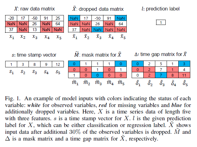
• \(M=\left\{m_{1}, m_{2}, \ldots, m_{T}\right\}\).

  • mask matrix whose element \(m_{t}^{i} \in\{0,1\}\)
  • \(m_{t}^{i}=1\) : observed
  • \(m_{t}^{i}=0\) : missing

• \(\tilde{X}\) : dropped matrix

  • generated by additionally dropping a portion of the observed variables from \(X\) to make model learn how to impute missing values
  • corresponding mask matrix : \(\tilde{M}\)

• \(\Delta=\left\{\delta_{1}, \delta_{2}, \ldots, \delta_{T}\right\}\) : time gap matrix

  • 의미 : time interval from the last observation for each variable of \(\tilde{X}\)

  • \(\delta_{t}^{i}\) : how long \(\tilde{x}^{i}\) has been missing consecutively until the \(t\)-th time step
  • \(\delta_{t}^{i}= \begin{cases}0 & \text { if } t=0 \\ s_{t}-s_{t-1}+\delta_{t-1}^{i} & \text { if } t>1, m_{t-1}^{i}=0 \\ s_{t}-s_{t-1} & \text { if } t>1, m_{t-1}^{i}=1\end{cases}\).

Goal : predicting \(l\) & \(X\), using \(\tilde{X}, \tilde{M}, \Delta\)

• propose an end-to-end GANs-based model , that performs (1) & (2) jointly

  • (1) missing value imputation

  • (2) down stream task ( reg / cls )

    ( mainly focus on classification problem )

4. Proposed Method

details of proposed methods

consists of 2 modules

• 1) imputation module
• 2) prediction module

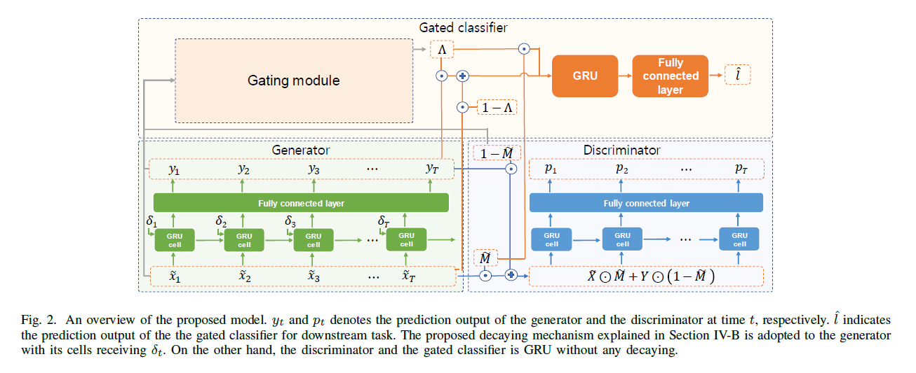
(1) Imputation using GAN

Wasserstein GAN

• \(G\) & \(D\) : GRU based RNNs

  • \(G\) : bidirectional RNN with decaying cell

    • input) \(x_{t}\)

    • output) same \(x_{t}\)

    • handle 2 kinds of input

      (1) observed ( \(m_t^i =1\) ) … \(G\) = auto encoder

      (2) missing ( \(m_t^i =0\) ) … reconstruct (X), estimate a new value (O)

Corrupted Data \(\tilde{X}\)

• obtained by randomly removing known variables given \(X\)

• \(\tilde{X} \sim \operatorname{Drop}_{\alpha}(\tilde{X} \mid X)\).

• ( dropout rate \(\alpha\) : hyperparameter )

• ( under missing rate \(r\) )

  randomly chosen \(100 \alpha \%\) of \(100(1-r) \%\) observed variables are dropped

Updated Mask Matrix \(\tilde{M}\)

• zero = denote where missing values are in \(\tilde{X}\) & artificially dropped values

\(r\) 이 크면, remove variable하는게 위험하다? NO!

\(\rightarrow\) 만약 corrupted 데이터가 아닌 raw 데이터에서만 온다면, generator cannot learn how to impute missing values!

따라서, propose DROPPING function!

• help the model to predict appropriate values for missing values

[ 요약 ] Generator

• (observed 데이터에 대해) auto-encoder
• (missing 데이터에 대해) authentic generator

Missing data : temporarily 다른 값으로 impute 되어 있어야

( 일단 input으로 넣긴 넣어야 하니까 )

• ex) 여기서는 mean imputation
• 따라서, input of \(G\) : \(Z=[\tilde{X} ;(1-\tilde{M})]\).

Loss Function

loss of \(G\) for reconstructing input :

• \(L_{G, r}=\mid \mid (G(Z)-X) \odot M \mid \mid _{F}^{2}\).

loss of \(G\) for minimizing adversarial loss :

• \(L_{D}=\mathbb{E}[D(G(Z)) \odot(1-\tilde{M})]+\mathbb{E}[-D(X) \odot \tilde{M}]\).
• \(L_{G, a}=\mathbb{E}[-D(G(Z)) \odot(1-\tilde{M})]\).

Final Loss for generator :

• \(L_{G}=L_{G, r}+\beta L_{G, a}\).

(2) Decaying mechanism for missing values

“Decaying” mechanism for generator

(previous method)

• common equation for \(\gamma_t\) ( = decaying rate, considering time gap )
• \(\gamma_{t}^{c}=\exp \left(-\max \left(0, W_{\gamma^{c}} \delta_{t}+b_{\gamma^{c}}\right)\right)\).

(proposed method)

previous method의 문제

• only uses \(t\)-th time gap,

  when measuring the decaying rate for \((t-1)\)-th hidden state vector

• fails to handle the temporal change of time gap values over time

제안한 방법

• decaying method that feeds \(k\) time gap vectors, \(\delta_{t-k+1: t}\)
• \(\eta_{t}=\max \left(0, W_{\eta} \delta_{t-k+1: t}+b_{\eta}\right)\).
• \(\gamma_{t}=\exp \left(-\max \left(\operatorname{Maxpool}\left(0, W_{\gamma} \eta_{t}^{T}+b_{\gamma}\right)^{T}\right)\right)\).

여러 패턴의 temporal time gap variations 있다는 가정 하에,

\(\rightarrow\) map \(\eta_t\) into 2-d space

introduce input decaying, that downscales input data \(\tilde{x_t}\) with the rate of \((1-\gamma_t)\)

[ 요약 ] update functions of GRU (with decaying mechanism)

\(\begin{gathered} h_{t-1}=\gamma_{t} \odot h_{t-1}, \quad z_{t}=\left[\left(1-\gamma_{t}\right) ; 0\right] \odot z_{t} \\ u_{t}=\sigma\left(W_{u}\left[h_{t-1} ; z_{t}\right]+b_{u}\right), \quad r_{t}=\sigma\left(W_{r}\left[h_{t-1} ; z_{t}\right]+b_{r}\right) \\ \tilde{h}_{t}=\tanh \left(W_{h}\left[r_{t} \odot h_{t-1} ; z_{t}\right]+b_{h}\right) \\ h_{t}=\left(1-u_{t}\right) \odot h_{t-1}+u_{t} \odot \tilde{h}_{t} \end{gathered}\).

(3) Gated Classifier & end-to-end multitask learning

introduce novel model, using gating mechanism, gated classifier \(C\)

• “considers the RELIABILITY of imputation results”

• mixes “observations” & “predictions” of imputation module

• ex) missing rate 높아 \(\rightarrow\) little info that we can extract to estimate its distribution

Gated Classifier의 gating module

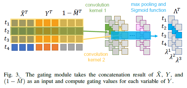
• 1) define a gating matrix \(\Lambda \in \mathbb{R}^{d \times T}\)

  ( 의미 : degree of reliability for \(Y\) ( = output of the generator) )

  ( 요소 : \(\lambda_{t}^{i} \in\{0,1\}\) )

• 2) use \(\tilde{X}\) & \(Y\) & \(\tilde{M}\) to estimate relative confidence of \(Y\) compared to \(\tilde{X}\)

  ( concatenate! \(\left[\tilde{X}^{T} ; Y^{T} ;\left(1-\tilde{M}^{T}\right)\right]^{T}\) …. \(3d \times T\) matrix )

• 3) compute convolution of above concatenation

  • mapping : \(\mathbb{R}^{3 d \times T} \rightarrow \mathbb{R}^{d \times T}\)

  • kernel size : \((3d, *)\)

    ex) kernel size = \((3d, 3)\) :

    \(\begin{gathered} {\left[\left[\tilde{x}_{t-1}^{T} ; y_{t-1}^{T} ;\left(1-\tilde{m}_{t-1}^{T}\right)\right]^{T}\right.} \\ {\left[\tilde{x}_{t}^{T} ; y_{t}^{T} ;\left(1-\tilde{m}_{t}^{T}\right)\right]^{T}} \\ \left.\left[\tilde{x}_{t+1}^{T} ; y_{t+1}^{T} ;\left(1-\tilde{m}_{t+1}\right)\right]^{T}\right] \end{gathered}\).

• 4) gating matrix \(\Lambda\) 만든 뒤,

  mix the “generator output” & “raw data” by gating value

  \(S=Y \odot \Lambda+\tilde{X} \odot(1-\Lambda)\).