[Paper Review] 22.(Analysis,Manipulation) LatentCLR ; A Contrastive Learning Approach for Unsupervised Discovery of Interpretable Directions

[Paper Review] 22. LatentCLR : A Contrastive Learning Approach for Unsupervised Discovery of Interpretable Directions

Contents

1. Abstract
2. Introduction
3. Related Work
   1. GAN
   2. Latent Space Navigation
4. Methodology
   1. Contrastive Learning
   2. Latent Contrastive Learning (LatentCLR)

0. Abstract

Possible to find interpretable directions in latent space of pre-trained GANs

• enable controllable image generation
• support a wide range of semantic editing operations

1. Introduction

introduce LatentCLR,

• optimization-based approach,
• that uses self-supervised contrastive objective to find interpretable directions in GANs
• use DIFFERENCES caused by an edit operation on the feature activations

Contribution

• use contrastive learning
• can find distinct & fine-grained directions on a variety of datasets

2. Related Work

1) GAN

most popular 1 : StyleGAN, StyleGAN2

• use a mapping network of 8-layer
• to map the input latent code to intermediate latent space

most popular 2 : BigGAN

• large-scale model trained on ImageNet

• also use intermediate layers,

  by using latent vector as input ( = skip-z inputs ), as well as class vectors

work with pre-trained StyleGAN2 & BigGANS

2) Latent Space Navigation

manipulate the latent structure of pre-trained GANs

• divided into 2 groups

[ (a) Supervised Setting ]

• use pre-trained classifiers, to guide optimization-based learning to discover interpretable directions
• ex) InterfaceGAN
  • benefit from labeled data ( ex. gender, facial expression, age .. )
• ex) GANalyze
  • find directions for cognitive image properties for a pre-trained BigGAN model, using an externally trained assessor function

[ (b) Unsupervised Setting ]

• skp

3. Methodology

preliminaries of contrastive learning

1) Contrastive Learning

• SOTA in unsupervised learning
• learn representations, by contrastive positive pairs against negative pairs
  • core idea :
    • similar pairs near
    • dissimilar pairs far
• this paper follows a similar approach to SimCLR

SimCLR

consists of 4 components

• 1) stochastic data augmentation
  • generates positive pairs \(\left(\mathrm{x}, \mathrm{x}^{+}\right)\)
• 2) encoding network \(f\)
  • extracts representation vectors out of augmented samples
• 3) small projector head \(g\)
  • maps representations to the loss space
• 4) contrastive loss function \(l\)
  • enforces the separation between positive and negative pairs

Given a random mini-batch of \(N\) samples…

• 1) generate \(N\) positive pairs
• 2) for all positive pairs, the remaining \(2(N-1)\) augmented samples are negative pairs
• 3) Notation
  • representations of all \(2N\) samples : \(\mathbf{h}_{i}=f\left(\mathbf{x}_{i}\right)\)
  • projections of \(\mathbf{h}_{i}\) : \(\mathbf{z}_{i}=g\left(\mathbf{h}_{i}\right)\)

• average of the NT-Xent loss over all positive pairs :

  • \(\ell\left(\mathbf{x}_{i}, \mathbf{x}_{j}\right)=-\log \frac{\exp \left(\operatorname{sim}\left(\mathbf{z}_{i}, \mathbf{z}_{j}\right) / \tau\right)}{\sum_{k=1}^{2 N} \mathbb{1}_{[k \neq i]} \exp \left(\operatorname{sim}\left(\mathbf{z}_{i}, \mathbf{z}_{k}\right) / \tau\right)}\).

    where \(\operatorname{sim}(\mathbf{u}, \mathbf{v})=\mathbf{u}^{T} \mathbf{v} / \mid \mid \mathbf{u} \mid \mid \mid \mid \mathbf{v} \mid \mid\) is cosine similariy

2) Latent Contrastive Learning (LatentCLR)

pre-trained GAN

• mapping function \(\mathcal{G}: \mathcal{Z} \rightarrow \mathcal{X}\)
• \(\mathrm{x}=\mathcal{G}(\mathbf{z})\).

edit directions

• directions \(\Delta \mathrm{z}\)
• such that the image \(\mathrm{x}^{\prime}=\mathcal{G}(\mathrm{z}+\Delta \mathrm{z})\) has semantically meaningful changes w.r.t \(\mathrm{x}\) , while preserving the identity of \(\mathrm{x}\).

limit ourselves to the unsupervised setting,

• where we aim to identify such edit directions without external supervision

• search for edit directions \(\Delta \mathbf{z}_{1}, \cdots, \Delta \mathbf{z}_{K}, K>1\), that have distinguishable effects in the target representation layer

Generalize directions, with potentially more expressive conditional mappings called direction models

Summary : consists of..

• 1) concurrent direction models
  • apply edits to given latent codes
• 2) target feature layer \(f\) of pre-trained GAN
  • evaluate direciton models
• 3) contrastive learning objective

Direction models

mapping \(\mathcal{D}\) : \(\mathcal{Z} \times \mathbb{R} \rightarrow \mathcal{Z}\)

• [INPUT] takes latent codes , along with a desired edit magnitude
• [OUTPUT] edited latent codes, i.e. \(\mathcal{D}:(\mathbf{z}, \alpha) \rightarrow \mathbf{z}+\Delta \mathbf{z}\), where \(\mid \mid \Delta \mathbf{z} \mid \mid \propto \alpha\).

3 alternative methods for direction model

• 1) global : \(\mathcal{D}(\mathbf{z}, \alpha)=\mathbf{z}+\alpha \frac{\theta}{ \mid \mid \theta \mid \mid }\)
• 2) linear : \(\mathcal{D}(\mathbf{z}, \alpha)=\mathbf{z}+\alpha \frac{\mathbf{M z}}{ \mid \mid \mathbf{M z} \mid \mid }\)
• 3) non-linear : \(\mathcal{D}(\mathbf{z}, \alpha)=\mathbf{z}+\alpha \frac{\mathbf{N} \mathbf{N}(\mathbf{z})}{ \mid \mid \mathbf{N} \mathbf{N}(\mathbf{z}) \mid \mid }\)

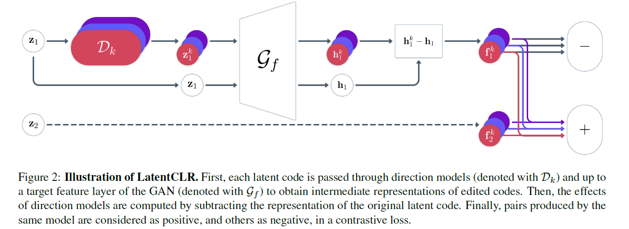
Target feature differences

Setting

• latent code \(\mathbf{z}_{i}, 1 \leq\) \(i \leq N\)
• mini-batch of size \(N\)
• \(K\) distinct edited latent codes : \(\mathbf{z}_{i}^{k}=\mathcal{D}\left(\mathbf{z}_{i}, \alpha\right)\)
• intermediate feature representations : \(\mathbf{h}_{i}^{k}=\mathcal{G}_{f}\left(\mathbf{z}_{i}^{k}\right)\)

Feature divergences

• \(\mathbf{f}_{i}^{k}=\mathbf{h}_{i}^{k}-\mathcal{G}_{f}\left(\mathbf{z}_{\mathbf{i}}\right)\).

Objective function

For each edited latent code \(\mathbf{z}_{i}^{k}\) :

\(\ell\left(\mathbf{z}_{i}^{k}\right)=-\log \frac{\sum_{j=1}^{N} \mathbb{1}_{[j \neq i]} \exp \left(\operatorname{sim}\left(\mathbf{f}_{i}^{k}, \mathbf{f}_{j}^{k}\right) / \tau\right)}{\sum_{j=1}^{N} \sum_{l=1}^{K} \mathbb{1}_{[l \neq k]} \exp \left(\operatorname{sim}\left(\mathbf{f}_{i}^{k}, \mathbf{f}_{j}^{l}\right) / \tau\right)}\).