(paper) An Empirical Evaluation of Generic Convolutional and Recurrent Networks for Sequence Modeling

An Empirical Evaluation of Generic Convolutional and Recurrent Networks for Sequence Modeling (2018)

Contents

1. Abstract
2. Introduction
3. Literature Review
   1. DL & Sequence Modeling
   2. Electricity Price Forecasting (EPF)
4. NBEATSx Model
   1. Stacks and Blocks
   2. Residual Connections

0. Abstract

sequence modleling \(\approx\) recurrent networks

recent results indicate that… “convolutional architecture outperforms RNN on tasks such as audio synthesis and machine translation”

Which one should we use??

\(\rightarrow\) this paper conducts systematic evaluation for the 2

1. Introduction

conduct a systematic empirical evaluation of

• 1) convolutional ( TCN )
• 2) recurrent ( LSTM, GRUs )

architectures on a broad range of sequence modeling task

Result : TCN > LSTM,GRUs

• not only in terms of accuracy
• but also simpler and clearer

2. TCN (Temporal Convolutional Networks)

characteristics of TCN

• 1) “casual” ( = no information leakage from future to past )
• 2) take a sequence of any length & map it to an output sequence of “same length”
• ( much simpler than WaveNet )
• ( do not use gating mechanisms & have much longer memory )

very long effective history sizes using a combination of ..

• 1) very DEEP networks ( + residual layers ) and
• 2) dilated convolutions

(1) Sequence Modeling

Sequence Modeling task?

• input sequence : \(x_{0}, \ldots, x_{T}\)

• wish to predict : \(y_{0}, \ldots, y_{T}\)

• constraint : to predict \(y_t\) …

  • only use \(x_0,...x_t\)

• sequence modeling network : \(f: \mathcal{X}^{T+1} \rightarrow \mathcal{Y}^{T+1}\)

  • \[\hat{y}_{0}, \ldots, \hat{y}_{T}=f\left(x_{0}, \ldots, x_{T}\right)\]

  • satisfies the causal constraint that \(y_t\) depends only on \(x_0,...x_t\)

    ( not on any future inputs! )

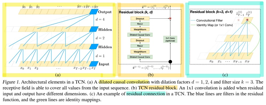
(2) Causal Convolutions

TCN is based upon 2 principles

• 1) uses a “1D fully convolutional network”
• 2) uses “causal convolutions”

TCN = 1D FCN + causal convolutions

Disadvantages

in order to achieve a long effective history size…

\(\rightarrow\) need an extremely deep network ( or very large filters )

(3) Dilated Convolutions

enable an exponentially large receptive field

Notation

• 1-D sequence input : \(\mathbf{x} \in \mathbb{R}^{n}\)

• filter : \(f:\{0, \ldots, k-1\} \rightarrow \mathbb{R}\)

• dilated convolution operation \(F\), on element \(s\) :

  \(F(s)=\left(\mathbf{x} *_{d} f\right)(s)=\sum_{i=0}^{k-1} f(i) \cdot \mathbf{x}_{s-d \cdot i}\).

  • \(d\) : dilation factor
  • \(k\) : filter size
  • \(s-d\cdot i\) : direction of the past

(4) Residual Connections

\(o=\operatorname{Activation}(\mathbf{x}+\mathcal{F}(\mathbf{x}))\).

3. Advantages & Disadvantages of TCN

Advantages

• 1) Parallelism ( both training & evaluation)
• 2) Flexible receptive size ( dilation factors & filter size )
• 3) stable gradients ( exploding/vanishing gradients (X) )
• 4) low memory requirement for training ( share filters across a layer )
• 5) variable length inputs

Distadvantages

• 1) data storage during evaluation

  • RNN : only maintain hidden state

    ( = summary of entire history )

  • TCN : take in the raw sequence up to the effective history length

• 2) potential parameter change for a transfer of domain