(paper) Temporal Fusion Transformers for Interpretable Multi-horizon Time Series Forecasting

Temporal Fusion Transformers for Interpretable Multi-horizon Time Series Forecasting (2020)

Contents

1. Abstract
2. Introduction
3. DeTSEC : Deep Time Series Embedding Clustering

0. Abstract

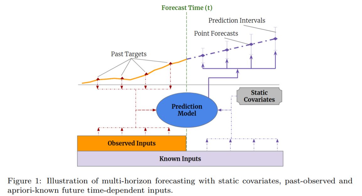
Multi-horizon forecasting

• often contains complex mix of inputs

Complex mix of Inputs

• 1) static covariates ( = time-invariant )

• 2) known future inputs

• 3) other exogenous time series

  ( = only observed in the past )

Most of DL = “black box”

Propose TFT ( = Temporal Fusion Transformer )

• novel attention-based architecture
• combines..
  • 1) high-performance multi-horizon forecasting
  • 2) with interpretable insights into temporal dynamics
• TFT uses..
  • 1) recurrent layers for local processing
  • 2) interpretable self-attention layers for long-term dependencies

1. Introduction

Multi-horizon forecasting

• prediction of multiple future time steps

have access to a variety of data

while, many architectures have focused on variants of RNN…. recent improvments have used ATTENTION-based methods ( ex. Transformer )

\(\rightarrow\) but fail to consider different types of inputs & assume that all exogenous inputs are known in the future

propose TFT

• an attention-based DNN architecture for multi-horizon forecasting
• achieves high performance while enabling new forms of interpretability

2. Related Work

2-1. DNNs for Multi-horizon Forecasting

categorized into..

• 1) [iterated approaches] using autoregressive models
• 2) [direct methods] based on seq2seq

[1] Iterated Approaches

• one-step ahead prediction models
• recursively feeding
• rely on assumption that all variables excluding target are known at forecast tiime
• [1] vs TFT
  • TFT : explicitly accounts for diversity of inputs

[2] Direct methods

• expliclity generate forecasts for multiple PRE-defined horizons at each time step
• usually rely on seq2seq
• [2] vs TFT
  • by interpreting attention patterns, TFT can provide insightful EXPLANATIONS about temporal dynamics

2-2. Time Series Interpretability with Attention

• attention : identify salient portions of input
• BUT… do not consider the IMPORTANCE of STATIC COVARIATES

TFT solves this by using SEPARATE encoder-decoder attention for static features

2-3. Instance-wise Variable Importances with DNNs

Instance-wise Variable Importances with DNNs :

• done by post-hoc explanations
• ex) LIME, SHAP, RL-LIM

TFT is able to analyze global temporal relationships and allows users to interpret global behaviors of the model on the whole dataset – specifically in the identification of any persistent patterns (e.g. seasonality or lag effects) and regimes present.

3. Multi-horizon Forecasting

Notation

• 1) static covariates : \(s_{i} \in \mathbb{R}^{m_{s}}\)
• 2) inputs : \(\chi_{i, t} \in \mathbb{R}^{m_{\chi}}\)
• 3) scalar targets : \(y_{i, t} \in \mathbb{R}\) at each time-step \(t \in\left[0, T_{i}\right]\). T

Time-dependent input features are subdivided into 2 categories

\(\chi_{i, t}=\left[\boldsymbol{z}_{i, t}^{T}, \boldsymbol{x}_{i, t}^{T}\right]^{T}\).

• \(\boldsymbol{z}_{i, t} \in \mathbb{R}^{\left(m_{z}\right)}\) : observed input
  • only be measured at each step & unknown beforehand
• \(\boldsymbol{x}_{i, t} \in \mathbb{R}^{m_{x}}\) : known inputs
  • can be predetermined

Prediction intervals

• adopt quantile regression to our multi-horizon forecasting setting
• (e.g. outputting the \(10^{t h}\), \(50^{t h}\) and \(90^{t h}\) percentiles at each time step)

Each quantile forecast takes the form :

\(\hat{y}_{i}(q, t, \tau)=f_{q}\left(\tau, y_{i, t-k: t}, \boldsymbol{z}_{i, t-k: t}, \boldsymbol{x}_{i, t-k: t+\tau}, s_{i}\right)\).

• \(q^{t h}\)sample quantile
• \(\tau\) step ahead forecast at time \(t\)
• \(f_{q}(.)\): prediction model

Simulatenously output forecasts for \(\tau_{max}\) time steps!

• i.e. \(\tau \in\) \(\left\{1, \ldots, \tau_{\max }\right\}\).
• incorporate all past information within a finite look-back window \(k\)

4. Model Architecture

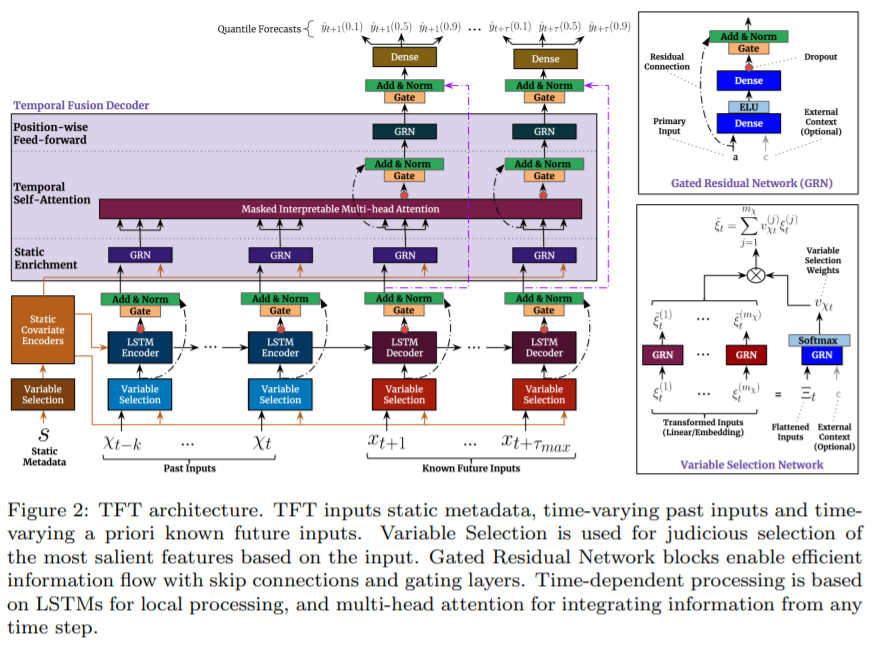
design TFT to use canonical components

• efficiently build feature representations for each input type

  ( static / known / observed )

4 major constituents of TFTS :

• 1) Gating mechanism
• 2) Variable selection networks
• 3) Static covariate encoders
• 4) Temporal processing
• 5) Prediction Intervals

4-1. Gating Mechanism

• relationship between exogenous inputs and targets
• propose GRN ( Gated Residual Network ) as building block of TFT
  • input 1) primary input \(\mathbf{a}\)
  • input 2) optional context vector \(c\)

\(\begin{aligned} \operatorname{GRN}_{\omega}(\boldsymbol{a}, \boldsymbol{c}) &=\text { LayerNorm }\left(\boldsymbol{a}+\operatorname{GLU}_{\omega}\left(\boldsymbol{\eta}_{1}\right)\right) \\ \boldsymbol{\eta}_{1} &=\boldsymbol{W}_{1, \omega} \boldsymbol{\eta}_{2}+\boldsymbol{b}_{1, \omega} \\ \boldsymbol{\eta}_{2} &=\operatorname{ELU}\left(\boldsymbol{W}_{2, \omega} \boldsymbol{a}+\boldsymbol{W}_{3, \omega} \boldsymbol{c}+\boldsymbol{b}_{2, \omega}\right) \end{aligned}\).

• use component gating layers, based on GLU (Gated Linear Units) to provide flexibility
  • \(\mathrm{GLU}_{\omega}(\boldsymbol{\gamma})=\sigma\left(\boldsymbol{W}_{4, \omega} \boldsymbol{\gamma}+\boldsymbol{b}_{4, \omega}\right) \odot\left(\boldsymbol{W}_{5, \omega} \boldsymbol{\gamma}+\boldsymbol{b}_{5, \omega}\right)\).
  • allows TFT to control the extent to which the GRN contributs to the original input \(\mathbf{a}\)

4-2. Variable Selection Networks

• multiple variables may be available

• instance wise variable selection
  • applied both to “static covariates” & “time-dependent covariates”
• learning capacity only on the most salient ones

(1) categorical variables : entity embeddings

(2) continuous variables : linear transformations

all static/past/future inputs make use of separate variable selection networks

\(\boldsymbol{\Xi}_{t}=\left[\boldsymbol{\xi}_{t}^{(1)^{T}}, \ldots, \boldsymbol{\xi}_{t}^{\left(m_{\chi}\right)^{T}}\right]^{T}\).

• \(\boldsymbol{\xi}_{t}^{(j)} \in \mathbb{R}^{d_{\text {model }}}\) : transformed input of the \(j\)-th variable at time \(t\).

Variable selection weights :

\(\boldsymbol{v}_{\chi_{t}}=\operatorname{Softmax}\left(\operatorname{GRN}_{v_{\chi}}\left(\boldsymbol{\Xi}_{t}, \boldsymbol{c}_{s}\right)\right)\).

( where \(\boldsymbol{v}_{\chi_{t}} \in \mathbb{R}^{m_{\chi}}\) is a vector of variable selection weights, )

• external context vector \(\boldsymbol{c}_{s}\)

additional layer of non-linear processing :

• \(\tilde{\boldsymbol{\xi}}_{t}^{(j)}=\operatorname{GRN}_{\tilde{\xi}(j)}\left(\boldsymbol{\xi}_{t}^{(j)}\right)\).

processed features : weighted average

• \(\tilde{\boldsymbol{\xi}}_{t}=\sum_{j=1}^{m_{\chi}} v_{\chi_{t}}^{(j)} \tilde{\boldsymbol{\xi}}_{t}^{(j)}\).

4-3. Static Covariate Encoders

integrate additional information! using separate GRN encoders

• 4 different context vectors : \(\mathbf{c}_s,\mathbf{c}_e,\mathbf{c}_c,\mathbf{c}_h\)

  ( wired into various locations in the temporal fusion decoder )

• \(\mathbf{c}_s\) : context for temporal variable selection

• \(\mathbf{c}_c,\mathbf{c}_h\) : context for local processing of temporal features

• \(\mathbf{c}_e\) : context for enriching of temporal features with static information

4-4. Interpretable Multi-head Attention

( 기존 )

\(\operatorname{MultiHead}(\boldsymbol{Q}, \boldsymbol{K}, \boldsymbol{V})=\left[\boldsymbol{H}_{1}, \ldots, \boldsymbol{H}_{m_{H}}\right] \boldsymbol{W}_{H}\).

• \(\boldsymbol{H}_{h}=\operatorname{Attention}\left(\boldsymbol{Q} \boldsymbol{W}_{Q}^{(h)}, \boldsymbol{K} \boldsymbol{W}_{K}^{(h)}, \boldsymbol{V} \boldsymbol{W}_{V}^{(h)}\right)\).

( 제안 )

\(\text { InterpretableMultiHead }(\boldsymbol{Q}, \boldsymbol{K}, \boldsymbol{V})=\tilde{\boldsymbol{H}} \boldsymbol{W}_{H}\).

• \(\begin{aligned} \tilde{\boldsymbol{H}}=& \tilde{A}(\boldsymbol{Q}, \boldsymbol{K}) \boldsymbol{V} \boldsymbol{W}_{V} \\ =&\left\{1 / H \sum_{h=1}^{m_{H}} A\left(\boldsymbol{Q} \boldsymbol{W}_{Q}^{(h)}, \boldsymbol{K} \boldsymbol{W}_{K}^{(h)}\right)\right\} \boldsymbol{V} \boldsymbol{W}_{V} \\ =& 1 / H \sum_{h=1}^{m_{H}} \operatorname{Attention}\left(\boldsymbol{Q} \boldsymbol{W}_{Q}^{(h)}, \boldsymbol{K} \boldsymbol{W}_{K}^{(h)}, \boldsymbol{V} \boldsymbol{W}_{V}\right) \end{aligned}\).
• where \(\boldsymbol{W}_{V} \in \mathbb{R}^{d_{\text {model }} \times d_{V}}\) are value weights shared across all heads

4-5. Temporal Fusion Decoder

(1) Locality Enhancement with seq2seq layer

• \(\tilde{\boldsymbol{\phi}}(t, n)=\text { LayerNorm }\left(\tilde{\boldsymbol{\xi}}_{t+n}+\operatorname{GLU}_{\tilde{\phi}}(\boldsymbol{\phi}(t, n))\right)\).

(2) static enrichment layer

• \(\boldsymbol{\theta}(t, n)=\operatorname{GRN}_{\theta}\left(\tilde{\boldsymbol{\phi}}(t, n), \boldsymbol{c}_{e}\right)\).
• \(c_e\) is a context vector from a static covariate encoder

(3) Temporal Self-attention layer

• all static-enriched temporal features are first grouped into single matrix

  \(\boldsymbol{\Theta}(t)=[\boldsymbol{\theta}(t,-k), \ldots,\).\(\boldsymbol{\theta}(t, \tau)]^{T}\)

• Interpretable Multi-head attention

  \(\boldsymbol{B}(t)=\operatorname{InterpretableMultiHead}(\boldsymbol{\Theta}(t), \boldsymbol{\Theta}(t), \boldsymbol{\Theta}(t))\).

• Decoder masking ( only attend to features preceding it )

• after self-attention layer…

  additional gating layer : \(\boldsymbol{\delta}(t, n)=\operatorname{LayerNorm}\left(\boldsymbol{\theta}(t, n)+\operatorname{GLU}_{\delta}(\boldsymbol{\beta}(t, n))\right)\).

(4) Position-wise FFNN

• \(\boldsymbol{\psi}(t, n)=\operatorname{GRN}_{\psi}(\boldsymbol{\delta}(t, n))\).

• \(\tilde{\boldsymbol{\psi}}(t, n)=\text { LayerNorm }\left(\tilde{\boldsymbol{\phi}}(t, n)+\operatorname{GLU}_{\tilde{\psi}}(\boldsymbol{\psi}(t, n))\right)\)>

4-6. Quantile Outputs

• simultaneous prediction of various percentiles (e.g. \(10^{\text {th }}, 50^{\text {th }}\) and \(\left.90^{t h}\right)\)

• generated using linear transformation of the output from the temporal fusion decoder:

  \(\hat{y}(q, t, \tau)=\boldsymbol{W}_{q} \tilde{\boldsymbol{\psi}}(t, \tau)+b_{q}\).

5. Loss Function

Quantile loss ( = summed across all quantile outputs )

\(\mathcal{L}(\Omega, \boldsymbol{W})=\sum_{y_{t} \in \Omega} \sum_{q \in \mathcal{Q}} \sum_{\tau=1}^{\tau_{\max }} \frac{Q L\left(y_{t}, \hat{y}(q, t-\tau, \tau), q\right)}{M \tau_{\max }}\).

• \(Q L(y, \hat{y}, q)=q(y-\hat{y})_{+}+(1-q)(\hat{y}-y)_{+}\).
• \(\Omega\) : the domain of training data containing \(M\) samples
• \(\boldsymbol{W}\) : weights of TFT
• \(\mathcal{Q}=\{0.1,0.5,0.9\}\).

for out-of-sample testing, evaluate the normalized quantile losses

\(q \text {-Risk }=\frac{2 \sum_{y_{t} \in \tilde{\Omega}} \sum_{\tau=1}^{\tau_{\max }} Q L\left(y_{t}, \hat{y}(q, t-\tau, \tau), q\right)}{\sum_{y_{t} \in \bar{\Omega}} \sum_{\tau=1}^{\tau_{\max }}\mid y_{t}\mid }\).