STFT with Python

STFT with Python

참고 : https://www.youtube.com/watch?v=fMqL5vckiU0&list=PL-wATfeyAMNrtbkCNsLcpoAyBBRJZVlnf

1. Import Packages

import os
import librosa
import librosa.display
import IPython.display as ipd
import numpy as np
import matplotlib.pyplot as plt

2. Import Dataset

scale_file = "audio/scale.wav"
debussy_file = "audio/debussy.wav"
redhot_file = "audio/redhot.wav"
duke_file = "audio/duke.wav"

listen to music!

ipd.Audio(redhot_file)

scale, sr = librosa.load(scale_file)
debussy, _ = librosa.load(debussy_file)
redhot, _ = librosa.load(redhot_file)
duke, _ = librosa.load(duke_file)

3. Extract STFT

• Frame size : size of the window
• Hop size : size of the window stride

FRAME_SIZE = 2048
HOP_SIZE = 512

• librosa.stft

S_scale = librosa.stft(scale, n_fft=FRAME_SIZE, hop_length=HOP_SIZE)
print(S_scale.shape)
print(type(S_scale[0][0]))

(1025, 342)
numpy.complex64

• 1025 : number of frequency bins
  • 1025 = (2048/2 + 1)
• 342 : number of frames

4. Calculate Spectogram

Scale : \(\mid S \mid^2\)

Y_scale = np.abs(S_scale) ** 2
print(Y_scale.shape)
print(type(Y_scale[0][0]))

(1025, 342)
numpy.float32

• taking magnitude => getting real number!

5. Visualization

def plot_spectrogram(Y, sr, hop_length, y_axis="linear"):
    plt.figure(figsize=(25, 10))
    librosa.display.specshow(Y, 
                             sr=sr, 
                             hop_length=hop_length, 
                             x_axis="time", 
                             y_axis=y_axis)
    plt.colorbar(format="%+2.f")

<br.

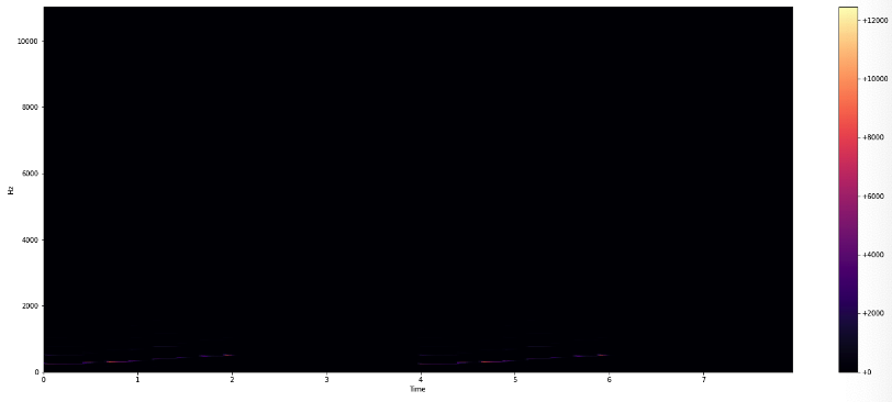
(1) Raw-scale

plot_spectrogram(Y_scale, sr, HOP_SIZE)

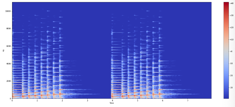
(2) Log-amplitude

Y_log_scale = librosa.power_to_db(Y_scale)
plot_spectrogram(Y_log_scale, sr, HOP_SIZE)

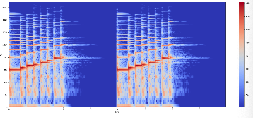
(3) Log-frequency

plot_spectrogram(Y_log_scale, sr, HOP_SIZE, y_axis="log")