TabTransformer; Tabular Data Modeling Using Contextual Embeddings

TabTransformer: Tabular Data Modeling Using Contextual Embeddings

https://arxiv.org/pdf/2012.06678.pdf

Contents

1. Introduction
2. The TabTransformer
3. Details of column embeddings
4. Pretraining the embeddings
5. Experiments
   1. Data
   2. Effectiveness of Transformer Layers
   3. The Robustness of TabTransformer
   4. Supervised Learning
   5. Semi-supervised Learning

Abstract

TabTransformer

• deep tabular model for SL & semi-SL
• use self-attention
• transform the embeddings of categorical features into robust contextual embeddings

Experiments

( with 15 publicly available datasets )

• outperforms the SOTA deep learning methods
• highly robust against both missing and noisy data features
• better interpretability
• for, semi-supervised setting … develop an unsupervised pre-training procedure

1. Introduction

SOTA of Tabular data: tree-based ensemble methods ( ex. GBDT )

• high prediction accuracy
• fast to train and easy to interpret

Limitations

• (1) Not suitable for continual training from streaming data
  • + Do not allow efficient end-to-end learning of encoders in presence of multi-modality along with tabular data.
• (2) In their basic form they are not suitable for SOTA semi-SL
  • \(\because\) basic decision tree learner does not produce reliable probability estimation to its predictions
• (3) SOTA methods of handling missing/noisy data is not applicable

MLP

• learn parametric embeddings to encode categorical features
• problem: shallow architecture & context-free embeddings
  • (a) neither the model nor the learned embeddings are interpretable
  • (b) it is not robust against missing and noisy data
  • (c) for semi-supervised learning, they do not achieve competitive performance
• Do not match the performance of tree-based models

To bridge this performance gap between MLP and GBDT..

\(\rightarrow\) various Deep Tabular methods have been proposed

• pros) achieve comparable prediction accuracy
• cons) do not address all the limitations of GBDT and MLP
  • + comparisons are done in a limited setting

TabTransformer

• address the limitations of MLPs and existing deep learning models

• bridge the performance gap between MLP and GBDT

• built upon Transformers to learn efficient contextual embeddings of categorical features

  • use of embeddings to encode words in a dense low dim space is prevalent in NLP

    ( = workd-token embeddings )

• experiment: fifteen publicly available datasets

2. The TabTransformer

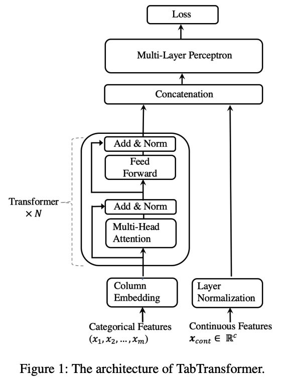
Architecture

1. Column embedding layer
2. Transformer layers ( x N )
   • multi-head self-attention + pointwise FFNN
3. MLP

Notation

\((\boldsymbol{x}, y)\) : feature-target pair

• where \(\boldsymbol{x} \equiv\) \(\left\{\boldsymbol{x}_{\mathrm{cat}}, \boldsymbol{x}_{\mathrm{cont}}\right\}\).
  • \(\boldsymbol{x}_{\mathrm{cat}} \equiv\left\{x_1, x_2, \cdots, x_m\right\}\) with each \(x_i\) being a categorical feature, for \(i \in\{1, \cdots, m\}\).

\(f_\theta\) : sequence of Transformer layers

Column Embedding

• embed each of the \(x_i\) categorical features into a parametric embedding of \(d\)-dim
• \(\boldsymbol{E}_\phi\left(\boldsymbol{x}_{\mathrm{cat}}\right)=\left\{\boldsymbol{e}_{\phi_1}\left(x_1\right), \cdots, \boldsymbol{e}_{\phi_m}\left(x_m\right)\right\}\) : set of embeddings for all the cat vars.
  • \(\boldsymbol{e}_{\phi_i}\left(x_i\right) \in \mathbb{R}^d\) for \(i \in\{1, \cdots, m\}\) .

\(\rightarrow\) These embeddings \(\boldsymbol{E}_\phi\left(\boldsymbol{x}_{\mathrm{cat}}\right)\) are inputted to the first Transformer layer

Sequence of Transformer layers: $f_\theta$.

( only for categorical variables )

• input: \(\left\{\boldsymbol{e}_{\phi_1}\left(x_1\right), \cdots, \boldsymbol{e}_{\phi_m}\left(x_m\right)\right\}\)
• output: contextual embeddings \(\left\{\boldsymbol{h}_1, \cdots, \boldsymbol{h}_m\right\}\)
  • where \(\boldsymbol{h}_i \in \mathbb{R}^d\) for \(i \in\{1, \cdots, m\}\).

Concatenate

• (1) contextual embeddings \(\left\{\boldsymbol{h}_1, \cdots, \boldsymbol{h}_m\right\}\)
• (2) continuous features \(\boldsymbol{x}_{\text {cont }}\)

\(\rightarrow\) vector of dim \((d \times m+c)\).

\(\rightarrow\) inputted to an MLP ( = \(g_\psi\) )

Loss Function

\(\mathcal{L}(\boldsymbol{x}, y) \equiv H\left(g_{\boldsymbol{\psi}}\left(f_{\boldsymbol{\theta}}\left(\boldsymbol{E}_\phi\left(\boldsymbol{x}_{\text {cat }}\right)\right), \boldsymbol{x}_{\text {cont }}\right), y\right)\).

• Cross Entropy: \(H\)

3. Details of column embedding

Embedding lookup table

• one embedding vector for one categorical variable
• \(\boldsymbol{e}_{\phi_i}(\).\() , for\) \(i \in\{1,2, \ldots, m\}\).

Example) \(i\) th feature with \(d_i\) classes

• embedding table \(\boldsymbol{e}_{\phi_i}\) has \(\left(d_i+1\right)\) embeddings
  • where the additional embedding corresponds to a missing value.
• The embedding for the encoded value \(x_i=j \in\left[0,1,2, . ., d_i\right]\) is \(\boldsymbol{e}_{\phi_i}(j)=\left[\boldsymbol{c}_{\phi_i}, \boldsymbol{w}_{\phi_{i j}}\right]\)
  • where \(\boldsymbol{c}_{\phi_i} \in \mathbb{R}^{\ell}, \boldsymbol{w}_{\phi_{i j}} \in \mathbb{R}^{d-\ell}\).
• unique identifier \(\boldsymbol{c}_{\phi_i} \in \mathbb{R}^{\ell}\)
  • act as column ID vector

Do not use positional encodings ( no order )

Appendix A

• ablation study on different embedding strategies
• different choices for \(\ell, d\) and element-wise adding the unique identifier and feature-value specific embeddings rather than concatenating them.

4. Pre-training the Embeddings

Self-SL

• Pre-training the Transformer layers using unlabeled data

• Fine-tuning :of the pre-trained Transformer layers along with the top MLP layer using the labeled data.

  • finetuning loss (same as above)
    • \(\mathcal{L}(\boldsymbol{x}, y) \equiv H\left(g_{\boldsymbol{\psi}}\left(f_{\boldsymbol{\theta}}\left(\boldsymbol{E}_\phi\left(\boldsymbol{x}_{\text {cat }}\right)\right), \boldsymbol{x}_{\text {cont }}\right), y\right)\).

2 types of pre-training procedures

• (1) MLM
• (2) RTD (replaced token detection)
  • replaces the original feature by a random value of that feature
  • Loss : binary CE … whether the feature has been replaced
  • uses auxiliary generator for sampling a subset of features

Why train auxiliary generator in NLP ?

• NLP) tens of thousands of tokens in language data

  \(\rightarrow\) uniformly random token is too easy to detect

• Tabular)

  • (1) the number of classes within each categorical feature is typically limited
  • (2) a different binary classifier is defined for each column rather than a shared one

5. Experiments

(1) Data

1. 15 binary CLS datasets ( from UCI )
2. AutoML challenge
3. Kaggle

for both SL & Semi-SL

Details:

• 5-fold CV splits
• train/val/test = 65:15:20
• # of cat vars: range from 2~136

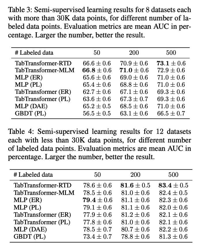
Semi-SL

• first \(p\) observation in training data are labeled
• the rest are unlabeled
• 3 scenarios: \(p \in \{50,200,500\}\).

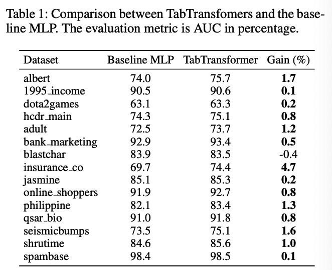
(2) Effectivenss of Transformer Layers

[ TabTransformer vs. MLP ]

Settings

• Supervised Learning
• MLP = TabTransformer - \(f_{\boldsymbol{\theta}}\)
  • TabTransforme w/o attention = MLP
• dimension of embeddings \(d\) for categorical features is set as 32 for both models

Results

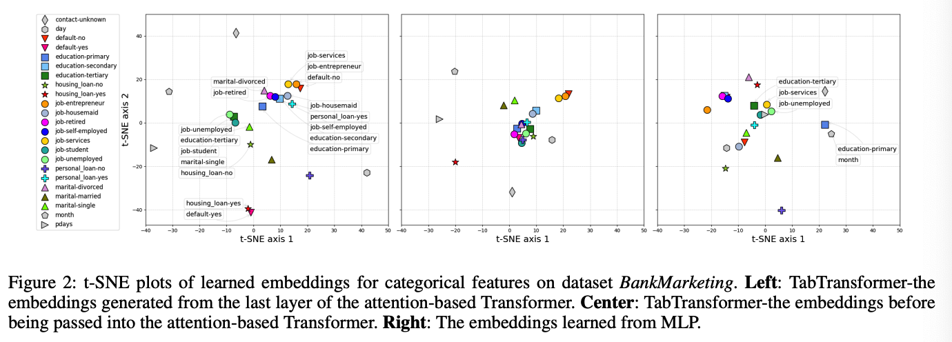
[ Contextual EMbeddings ]

from different layers of Transformer

(1) t-SNE plot

• with test dataset

• extract all contextual embeddings (across all columns) from a certain layer of the Transformer

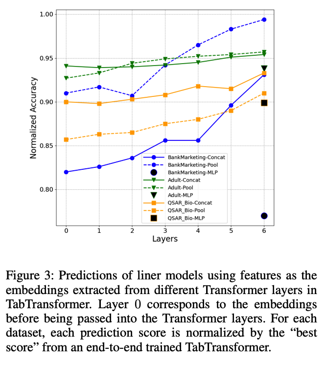
(2) Linear evaluation

• take all of the contextual embeddings of test data from each Transformer layer of a trained TabTransformer & use the embeddings from each layer along with the continuous variables as features \(\rightarrow\) then, separately fit a linear model with target \(y\). ( via logistic regression )

• motivation : simple linear model as a measure of quality for the learned embeddings.

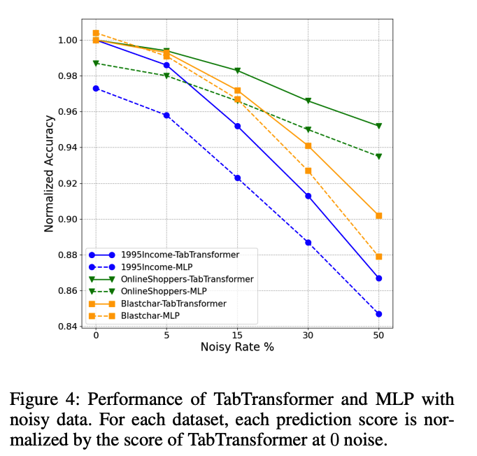
(3) The Robustness of TabTransformer

Noisy data & Data with missing values ( vs. MLP )

• only on categorical features, to specifically prove the robustness of contextual embeddings

a) Noisy Data

• (1) replace certain portion of values by randomly generated ones
  • from the corresponding columns (features).
• (2) pass into a trained TabTransformer to compute a prediction AUC score

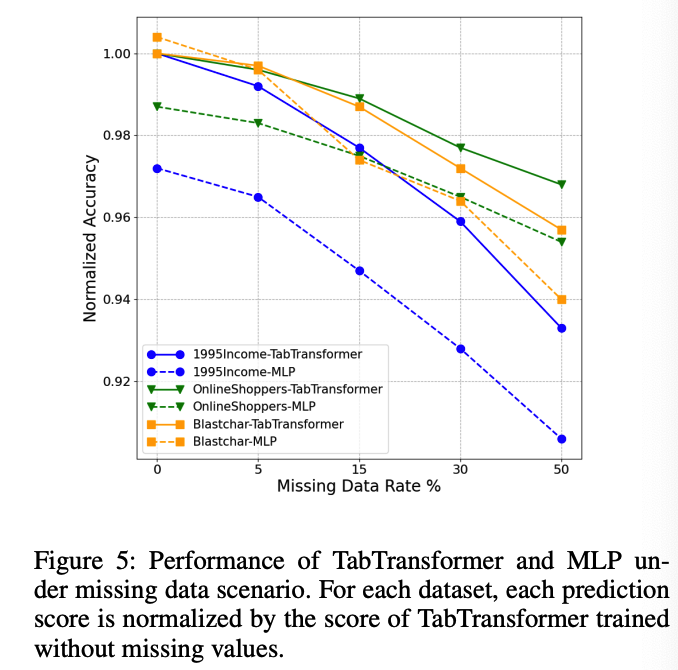
b) Data with Missing Values.

• (1) artificially select a number of values to be missing
• (2) send the data with missing values to a trained TabTransformer
  • 2 options to handle the embeddings of missing values
    • a) Use the average learned embeddings over all classes
    • b) embedding for the class of missing value ( in Section 2 )

( + Since the benchmark datasets do not contain enough missing values to effectively train the embedding in option (2), we use the average embedding in (1) for imputation )

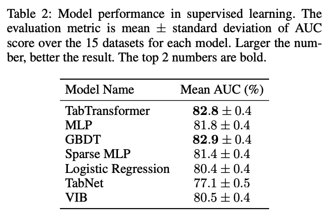
(4) Supervised Learning

compare with 4 categories of methods

• (1) Logistic Regression & GBDP
• (2) MLP & sparse MLP
• (3) TabNet
• (4) VIB

(5) Semi-supervised Learning