Toward Enhancing TS Contrastive Learning; A Dynamic Bad Pair Mining Approach

Toward Enhancing TS Contrastive Learning: A Dynamic Bad Pair Mining Approach

Contents

1. Abstract
2. Introduction
3. Related Work
4. CL in TS
5. Methods
   1. Problem Definition
   2. Analysis: TS CL
   3. Empirical Evidence
   4. DBPM
   5. Training
6. Experiments
   1. Linear Evaluation
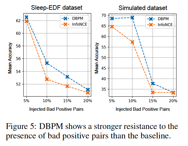
   2. Robustness against Bad Positive Pairs

Abstract

Not all positive pairs are beneficial to TS CL

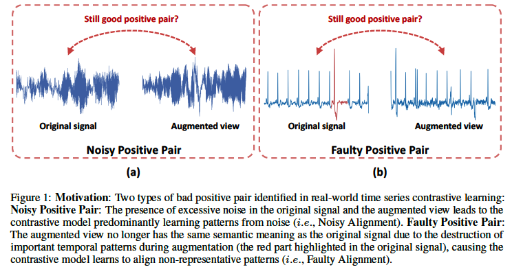
2 Types of bad positives

• (1) Noisy positive pair
  • Noisy Alignment: model tends to simply learn the pattern of noise
• (2) Faulty positive pair
  • Faulty Alignment: model wastes considerable amount of effort aligning non-representatitive patterns

Solution: Dynamic Bad Pair Mining (DBPM)

• Identifies & suppresses bad positive pairs in TS

• Memory module

  • to dynamically track the training behaviour of each positive pair

  • allows to find potential bad positive pairs at each epoch

    ( based on their historical training behaviors )

• Plug-in without additional parameters

1. Introduuction

Existing CL: assume that augmented views frorm same instances share meaning ful semantic info

\(\rightarrow\) What if violated?? ( = do not share meaningful info)

# Case 1) Noisy Positive Pairs ( Figure 1-(a) )

• Original signal = significant noise
• Result: shared info btw views is predominantly noise

# Case 2 Faulty Positive Pairs ( Figure 1-(b) )

• DA may impair spohisticated temporal patterns

Intuitive solution: suppress bad positive pairs

Problem: directly identifying bad positive pairs is challenging for 2 reasons

• (1) For noisy positive pairs, infeasible to measure the noise level
• (2) For faulty positive pairs, one will not be able to identify if the semantic meaning of augmented views are changed without the ground truth.

Investigate the training behavior of CL models with the presence of bad positive pairs using simulated data

• construct a simulated dataset: 3 pre-defined positive pair types
  • a) normal
  • b) noisy
  • c) faulty
• to explore the contrastive model’s reaction (i.e., training loss) to bad positive pairs.

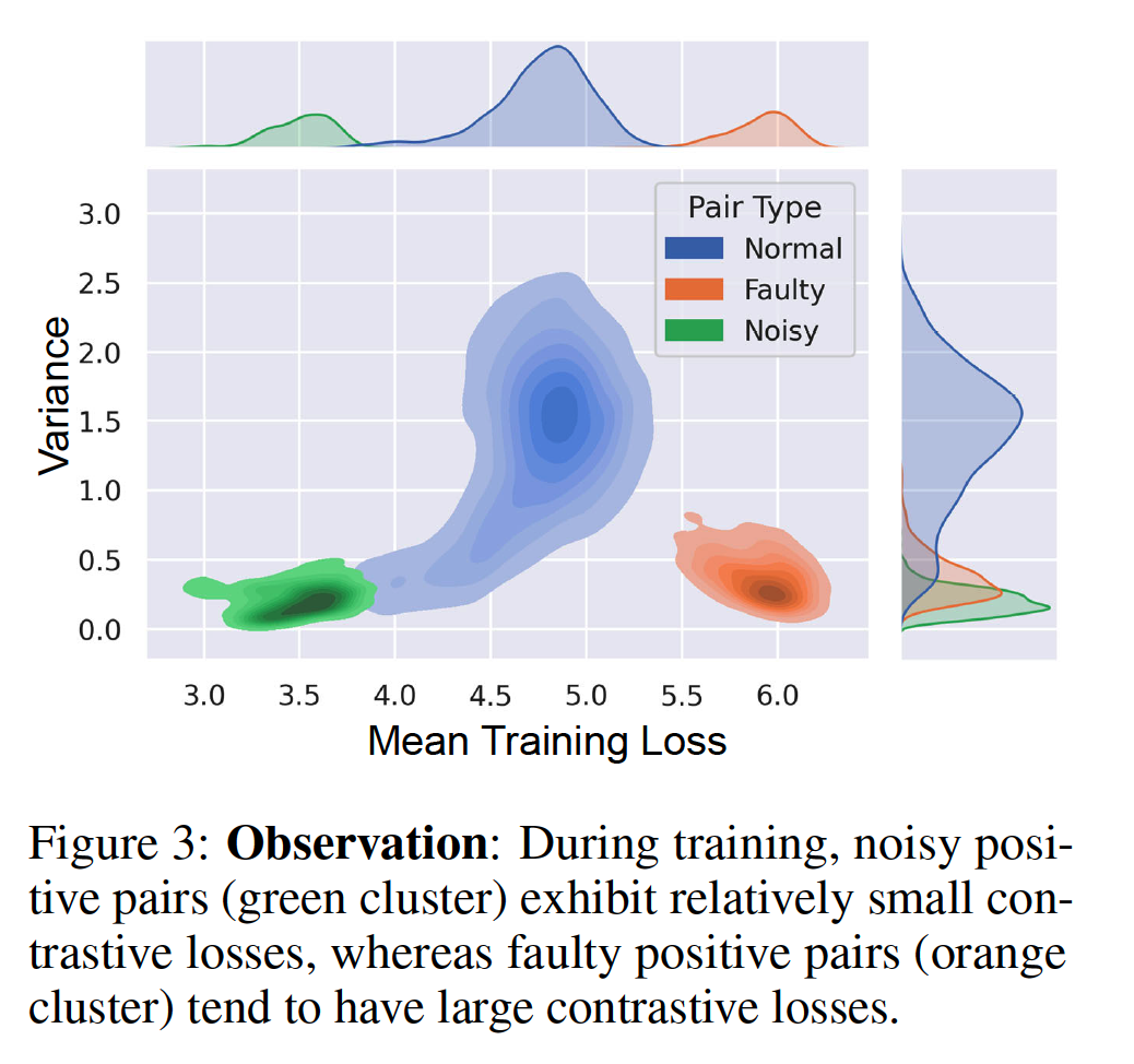
• (1) NOISY = small loss
• (2) FAULTY = large loss

Dynamic Bad Pair Mining (DBPM)

Key concept: (1) Identify & (2) Suppress

• (1) Identify: reliable bad positive pair mining
  • use memory module
    • high CL loss = more likely to be faulty positive pair
• (2) Suppress: down-weighting in CL
  • use transformation module
    • estimate suppressingg weight for bad positive pairs

2. Related Work

(1) Faultiy Positive Pairs in CV

• RINCE (Chuang, 2022)
  • symmetrical InfoNCE loss robust to faulty views
• Weighted xID
  • down-weight the suspicious audio-visual pairs

Difference of DDPM

• (1) Designed for TS domain
  • not only faultiy positive, but also noisy positive
• (2) Identifies bad positive pairs based on their historical training behaviors

(2) CL in TS

pass

(3) Learning with Label Error

pass

3. Methods

1) Drawbacks of current TS CL

2) Simulated Data

3) DBPM algorrithm

(1) Problem Definition

• TS: \(x \in \mathbb{R}^{C \times K}\)
• Encoder: \(G(\theta)\)

(2) Analysis: TS CL

Two views: \(\left(\boldsymbol{r}_i^u, \boldsymbol{r}_i^v\right)=\left(G\left(u_i \mid \theta\right), G\left(v_i \mid \theta\right)\right)\)

a) Noisy Alignment

Noisy positive pair problem

• Input data: \(x_i=z_i+\xi_i\),
  • where \(z_i \sim \mathcal{D}_z\) denotes the true signal and \(\xi_i \sim \mathcal{D}_{\xi}\) is the spurious dense noise
• Hypothesis: noisy positive pair problem is likely to occur on \(x_i\) when \(\xi_i \gg z_i\),
• Define \(\left(u_i, v_i\right)\) as a noisy positive pair when \(\xi_i^u \gg z_i^u\) and \(\xi_i^v \gg z_i^v\).

When noisy positive pairs present, \(\arg \max _\theta\left(I\left(G\left(u_i \mid \theta\right) ; G\left(v_i \mid \theta\right)\right)\right)\) is approximate to \(\arg \max _\theta\left(I\left(G\left(\xi_i^u \mid \theta\right) ; G\left(\xi_i^v \mid \theta\right)\right)\right)\).

\(\rightarrow\) Noisy alignment ( where the model predominantly learning patterns from noise )

b) Faulty Alignment

Faulty positive pair problem

• It is possible that random data augmentations alter or impair the semantic information, thus producing faulty views.
• Define \(\left(u_i, v_i\right)\) as a faulty positive pair when \(\tau\left(x_i\right) \sim \mathcal{D}_{\text {unknown }}\), where \(\mathcal{D}_{\text {unknown }} \neq \mathcal{D}_z\).

Partial derivatives of \(\mathcal{L}_{\left(u_i, v_i\right)}\) w.r.t. \(\boldsymbol{r}_i^u\)

• \(-\frac{\partial \mathcal{L}}{\partial \boldsymbol{r}_i^u}=\frac{1}{t}\left[\boldsymbol{r}_i^v-\sum_{j=0}^N \boldsymbol{r}_j^{v-} \frac{\exp \left(\boldsymbol{r}_i^{u \top} \boldsymbol{r}_j^{v-} / t\right)}{\sum_{j=0}^N \exp \left(\boldsymbol{r}_i^{u \top} \boldsymbol{r}_j^{v-} / t\right)}\right]\).

• Meaining)

  • Representation of augmented view \(u_i\) depends on the representation of augmented view \(v_i\), and vice versa.

    ( = Two augmented views \(u_i\) and \(v_i\) provide a supervision signal to each other )

Hypothesis: Rrom faulty positive pairs often exhibit low similarity (i.e., \(\left.\boldsymbol{s}\left(\boldsymbol{r}_i^u, \boldsymbol{r}_i^v\right) \downarrow\right)\), as their temporal patterns are different.

( = encoder will place larger gradient on faulty positive pairs, which exacerbates the faulty alignment )

(3) Empirical Evidence

• Figure 3 above

(4) DBPM

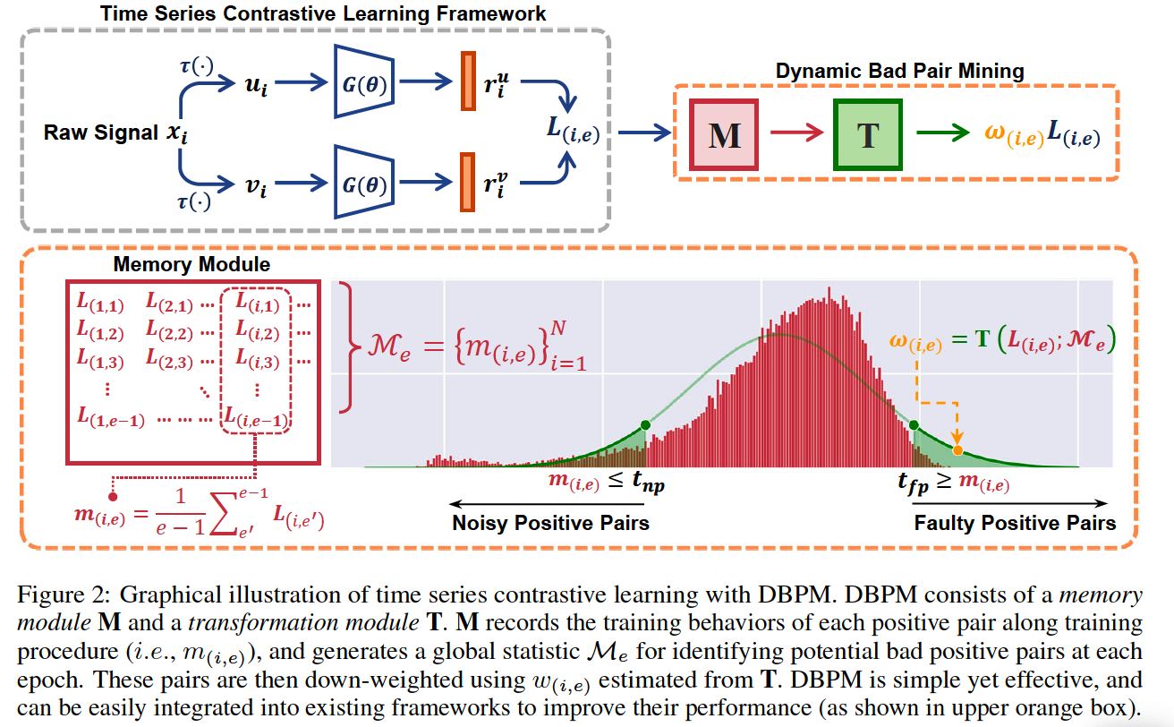
a) Identification

Memory module \(\mathbf{M} \in \mathbb{R}^{N \times E}\)

• To track individual training behavior at each training epoch
• Look-up table
  • \(N\) : the number of training samples
  • \(E\) : the number of maximum training epoch

<br.

For \(i\)-th positive pair \(\left(u_i, v_i\right)\)…

• \(\mathbf{M}_{(i, e)}\) is updated with its contrastive loss \(\mathcal{L}_{(i, e)}\) at \(e\)-th training epoch
• \(m_{(i, e)}=\frac{1}{e-1} \sum_{e^{\prime}=1}^{e-1} \mathcal{L}_{\left(i, e^{\prime}\right)}\).

Summarize the historical training behavior of \(i\)-th pair

• Mean training loss of \(\left(u_i, v_i\right)\) before \(e\)-th epoch \((e>1)\)
• At \(e\)-th training epoch …
  • \(\mathbf{M}\) will generate a global statistic \(\mathcal{M}_e=\left\{m_{(i, e)}\right\}_{i=1}^N\)
  • Use its mean and standard deviation as the descriptor for the global statistic at \(e\)-th epoch:
    • \(\mu_e=\frac{1}{N} \sum_{i=1}^N m_{(i, e)}\).
    • \(\sigma_e=\sqrt{\frac{\sum_{i=1}^N\left(m_{(i, e)}-\mu_e\right)^2}{N}}\).

To identify potential bad positive pairs, determine a threshold

• that differentiates them from normal positive pairs
• \(t_{n p}=\mu_e-\beta_{n p} \sigma_e, \quad t_{f p}=\mu_e+\beta_{f p} \sigma_e\).

b) Weight Estimation

Transformation module \(\mathbf{T}\)

• To estimate suppression weights for bad positive pairs at each training epoch
• \(w_{(i, e)}= \begin{cases}1, & \text { if } \mathbb{1}_i=0 \\ \mathbf{T}\left(\mathcal{L}_{(i, e)} ; \mathcal{M}_e\right), & \text { if } \mathbb{1}_i=1,\end{cases}\).
  • where \(\mathbb{1}_i\) is a indicator that is set to 1 if \(i\)-th pair is bad positive pair, 0 otherwise
• Maps the training loss of \(i\)-th positive pair at \(e\)-th epoch into a weight \(w_{(i, e)} \in(0,1)\).
• Set \(\mathbf{T}\) as a Gaussian pdf
  • \(\mathbf{T}\left(\mathcal{L}_{(i, e)} ; \mathcal{M}_e\right)=\frac{1}{\sigma_e \sqrt{2 \pi}} \exp \left(-\frac{\left(\mathcal{L}_{(i, e)}-\mu_e\right)^2}{2 \sigma_e^2}\right)\).

(5) Training

\(\mathcal{L}_{(i, e)}= \begin{cases}\mathcal{L}_{(i, e)}, & \text { if } \mathbb{1}_i=0 \\ w_{(i, e)} \mathcal{L}_{(i, e)}, & \text { if } \mathbb{1}_i=1\end{cases}\).

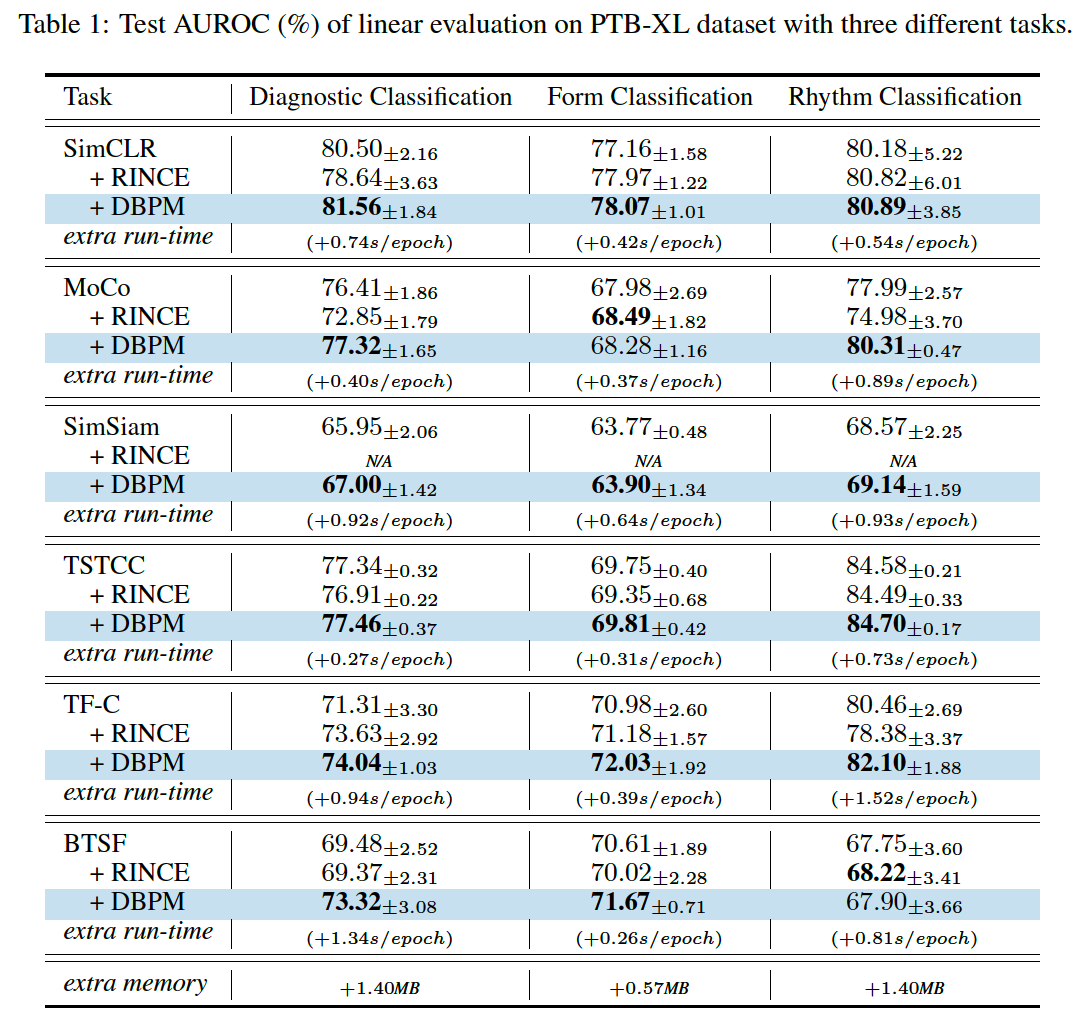
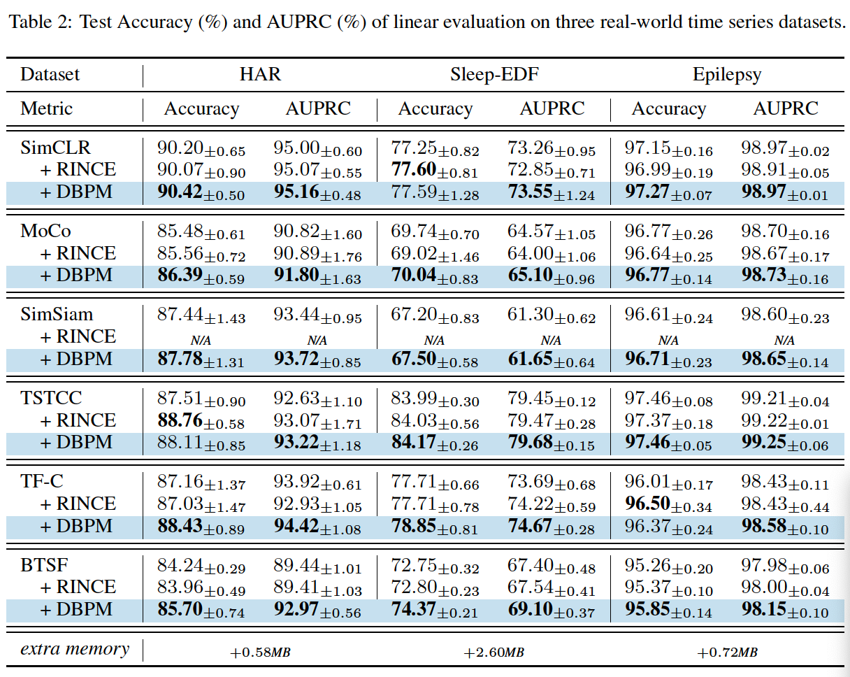
4. Experiments

(1) Linear Evaluation

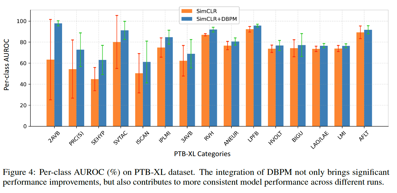
(2) Robustness against Bad Positive Pairs