(paper) Leaves; Learning Views for TS Data in Contrastive Learning

Leaves: Learning Views for TS Data in Contrastive Learning

( https://openreview.net/pdf?id=f8PIYPs-nB )

Contents

1. Abstract
2. Introduction
3. Related Works
   1. Augmentation-based Cl
   2. Automatic Augmentation
4. Methods
   1. LEAVES
   2. Adversarial Training

0. Abstract

Many CL methods : depend on data augmentations (DA)

• DA = generate different views from the original signal

Problem : tuning policies & hyper-parameters : time consuming

View-learning method :

• not well developed for TS data

LEAVES

Propose a simple but effective module for automating view generation for time-series data in CL

• learns the hyper-parameters for augmentations using adversarial training in CL

1. Introduction

DA methods : usually empirical

\(\rightarrow\) it remains an open question how to effectively generate views for a new dataset.

Instead of using artificially generated views … generate optimized views for the input samples

• ex) Tamkin et al. (2020) : ViewMaker
  • an adversarially trained convolutional module in CL to generate augmentation for images
  • problem : not utilized on TS data
    • TS signal : need to not only disturb the (1) magnitudes (spatial) but also distort the (2) temporal dimension

LEAVES

• lightweight module for learning views on TS data in CL
• optimized adversarially against the contrastive loss to generate challenging views
• propose TimeDistort
  • differentiable data augmentation technique for TS
  • to introduce smooth temporal perturbations to the generated views

example) generated views of ECG from ViewMaker & LEAVES

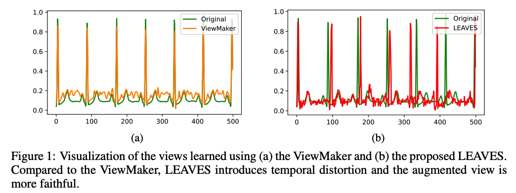
Viewmaker

• no temporal location is perturbed
• flat region of the original ECG signal was completely distorted.

LEAVES

• can distort the original signal in both spatial & temporal domains
• redue the risk of losing intact information due to excessive perturbation in time-series data.

Summary

• proposed LEAVES outperforms the baselines, including SimCLR and the SOTA methods

• generates more reasonable views compared to the SOTA methods in TS

2. Related Works

(1) Augmentation-based CL

DA plays essential roles in generating views

Many CL frameworks : developed based on the image transformation in CV

• ex) SimCLR, BYOL, Barlo Twin,

CL in TS domain

• ex) Gopal et al. (2021) : clinical domain-knowledge-based augmentation on ECG data and generated views from ECG from contrastive learning.
• ex) Mehari & Strodthoff (2022) : applied well-evaluated methods such as SimCLR, BYOL, and CPC Oord et al. (2018) on time-series ECG data for clinical downstream tasks.
• ex) Wickstrøm et al. (2022) : generated contrastive views by applying the MixUp augmentation in TS

However, the empirically augmented views might not be optimal

\(\rightarrow\) as exploring appropriate sets of augmentations is expensive.

(2) Automatic Augmentaiton

Methods of optimizing the appropriate augmentation strategies

• ex) AutoAugment (Cubuk et al., 2019)
  • designed as a RL based algorithm to search augmentation policies
  • including the “possibility” and “order” of using different augmentation methods.
• ex) DADA (Li et al., 2020)
  • gradient-based optimization strategy
  • find the augmentation policy with the highest probabilities after training,
    • which significantly reduces the search time compared to algorithms such as AutoAugment

these have been proven to have high performance

\(\rightarrow\) BUT require heavy computational complexity

Instead of searching for augmentations from the policy space…

\(\rightarrow\) learn views !!

• can be understood as generating data transformation by NN, raher than using manually tuned augmentations
• ex) Rusak et al. (2020)
  • applied a CNN to generate noise based on the input data and trained the perturbation generator in an adversarial manner against the supervised loss
• ex) Tamkin et al. (2020)
  • proposed a ResNet-based ViewMaker
  • to generate views for data for the CL
  • training of ViewMaker was also adversarial by maximizing the contrastive loss against the objective of the representation encoder.

these methods lack consideration of temporal perturbation when used in TS data

LEAVES

generate both the (1) magnitude and (2) temporal perturbations in sequences.

3. Methods

use SimCLR architecture

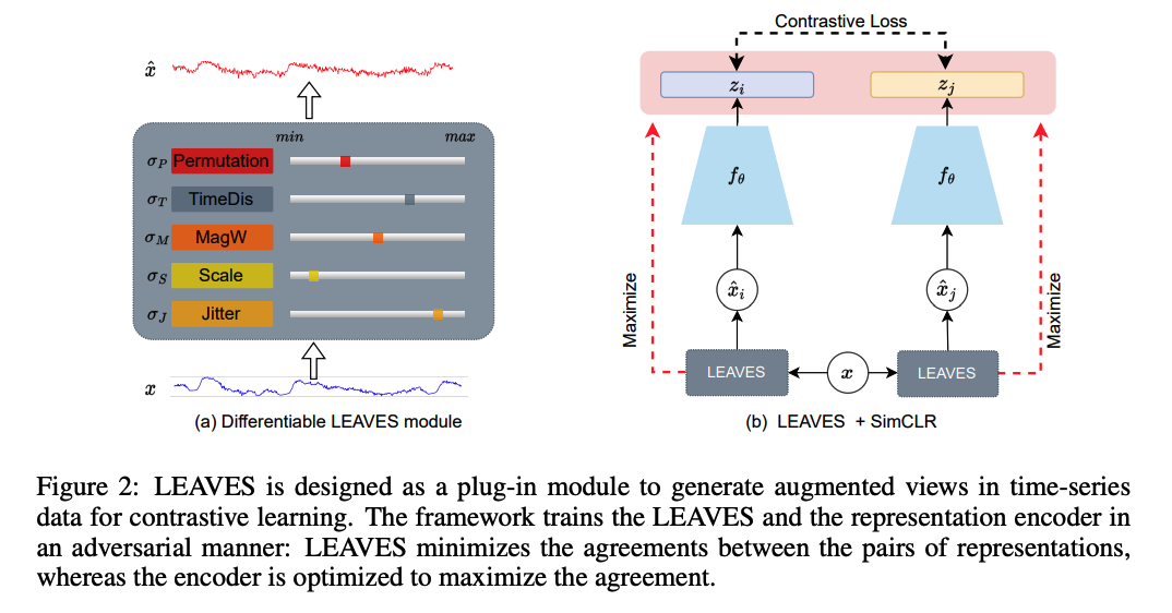
• overview of the pre-training architecture.
• step 1) differentiable LEAVES module,
  • can generate more challenging but still faithful views of an input.
• step 2) plugged into the SimCLR framework
• trained with the encoder in an adversarial manner.

(1) LEAVES

easily plugged into the CL

consists of a series of differentiable data augmentation methods, including …

• Jitter \(T_J\), Scale \(T_S\), magnitude warping (MagW) \(T_{M W}\), permutation (Perm) \(T_P\), and a newly proposed method named time distortion (TimeDis) \(T_{T D}\).

Notation : \(T_J \odot T_P\)

• step 1) jittering noise
• step 2) permutation

Proposed module generates view \(\hat{X}\) by… \(\hat{\mathbf{X}}=\mathbf{X} \odot T_J\left(\sigma_J\right) \odot T_S\left(\sigma_S\right) \odot T_{M W}\left(\sigma_M\right) \odot T_{T D}\left(\sigma_T\right) \odot T_P\left(\sigma_P\right)\)

• \(\sigma\) : represents the hyper-parameters of the DA
  • ex) \(\sigma_J\) : std of jittering noise
  • target learning parameters of this module are the \(\sigma\) of augmentation methods.

By learning \(\sigma\) …

• learns the strategy of generating views by combining multiple augmentation methods

• do not deliberately tune the order of augmentations applied to \(X\) in equation 1

  ( \(\because\) as the hyper-parameters and views of augmentations are independent )

a) Differentiable DA for TS data

ex) Jitter, Scale, and MagW

• perturb the magnitude of the original signal

ex) time warping (TimeW) and Perm

• corrupt the temporal location.

To optimize the hyper-parameters in these augmentation …

\(\rightarrow\) gradients are needed to be propagated back to these parameters during the training process.

However, these augmentation methods are based on non-differentiable operations such as drawing random values

\(\rightarrow\) Reparameterization tricks ( except the TimeW )

• TimeW : indexing operation makes it difficult to retrieve gradients.

propose the TimeDis augmentation

• to smoothly distort temporal information

Examples

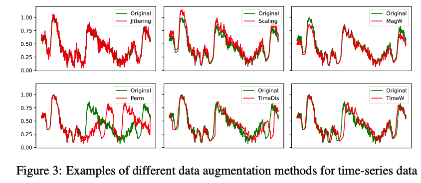
• six augmentation methods on TS
• constrain the noise with an up-bound…
  • \(\eta\) : maximum values of \(\sigma\) values in magnitude-based methods ( Jitter, Scale, MagW )
  • \(K\) : maximum segments ( Perm )

TimeDis

• relies on a smooth probability distribution to generate the probability of the location to be sampled in the original signal.

• utilize a reparameterized GMM with \(M\) Gaussian components as \(\sum_i^M \phi_i \mathcal{N}\left(\mu_i, \sigma_i^2\right)\)

  • to generate the location indexes \(\lambda \in \mathbb{R}^{N \times C \times L}\) from -1 to 1.

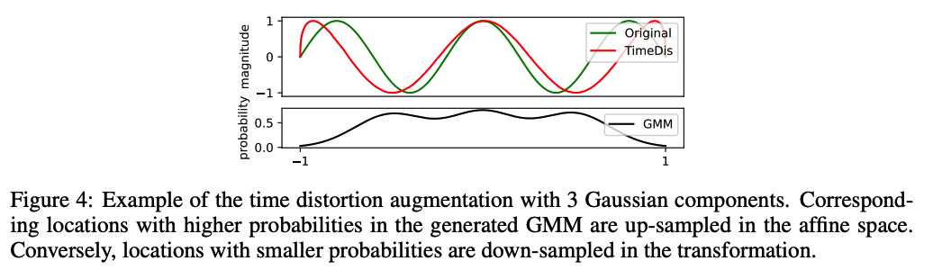
• -1 : first time step (position 1)
• 1 : last time step (position \(L\) )
• use \(\lambda\) to affine the original signal \(X\) as the view \(\hat{X}\),
  • locations with dense indexes in \(\lambda\) : the intervals among samples become looser;
  • locations with sparse indexes in \(\lambda\) : the corresponding intervals would be tighter.

(2) Adversarial Training

SimCLR

\(\begin{gathered} \mathcal{L}=\frac{1}{2 N} \sum_{k=1}^N[\ell(2 k-1,2 k)+\ell(2 k, 2 k-1)] \\ \ell_{i, j}=-\log \frac{\exp \left(s\left(z_i, z_j\right) / \tau\right)}{\sum_{k=1}^{2 N} \mathbb{1}_{k \neq i} \exp \left(s\left(z_i, z_k\right) / \tau\right)} \end{gathered}\).

LEAVES & encoder : optimized in opposite directions:

• encoder : minimize \(\mathcal{L}\)
• LEAVES : maximize \(\mathcal{L}\).