(paper) Soft Neighbors are Positive Supporters in Contrastive Visual Representation Learning

Soft Neighbors are Positive Supporters in Contrastive Visual Representation Learning

( https://openreview.net/pdf?id=l9vM_PaUKz )

Contents

1. Abstract
2. Introduction
3. Related Works
   1. Self-supervised visual representation learning
   2. Nearest neighbor exploration in visual recognition
4. Proposed Method
   1. Revisiting CL
   2. SNCLR (Soft Neighbors CL)

0. Abstract

Binary instance discrimination in CL

\(\rightarrow\) binary instance labeling is insufficient to measure correlations between different samples.

Propose to support the current image by exploring other correlated instances (i.e., soft neighbors).

soft neighbor contrastive learning method (SNCLR)

step 1) cultivate a candidate neighbor set

• will be further utilized to explore the highly-correlated instances.

step 2) cross-attention module

• predict the correlation score (denoted as positiveness) of other correlated instances with respect to the current one.

• positiveness score
  • measures the positive support from each correlated instance
• encoded into the objective for pretext training.

1. Introduction

CL : ceate multiple views based on different DAs

• These views are passed through a two-branch pipeline for similarity measurement
• ex) InfoNCE, redundancy-reduction loss
• Created views :
  • assigned with binary labels ( pos (1) & neg (0) )

Observe that this binary labels are not sufficient to represent instance correlations

• Without original training labels, contrastive learning methods are not effective in capturing the correlations between image instances.

• The learned feature representations are limited to describing correlated visual contents across different images.

Exploring Instance correlations

• ex) SwAV (Caron et al., 2020) and NNCLR (Dwibedi et al., 2021)

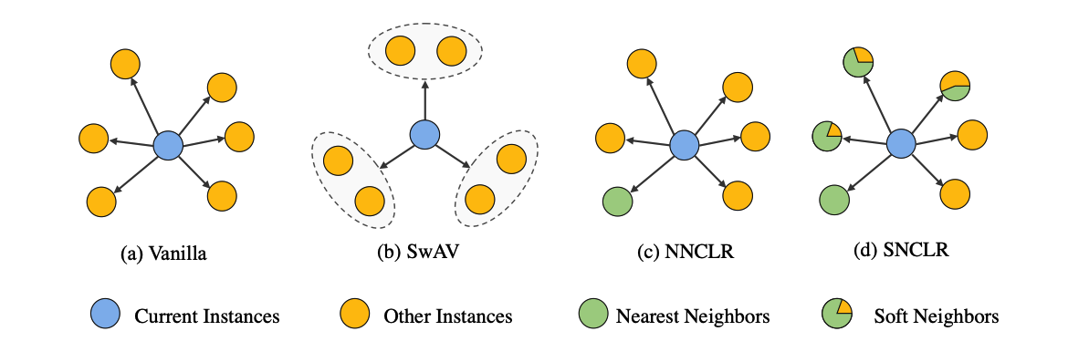
(a) vanilla CLR method

(b) SwAV

• assigns view embeddings of the current image instance to neighboring clusters.
• The contrastive loss computation is based on these clusters rather than view embeddings.

(c) NNCLR

• nearest neighbor (NN) view embeddings are utilized
• to support the current views to compute the contrastive loss.

(d) SNCLR

• aim to accurately identify the neighbors that are highly correlated to the current image instance, which is inspired by the NN selection.
• expect to produce a soft measurement of the correlation extent, which is motivated by the clustered CLR.

SNCLR

• propose to explore “soft” neighbors during CL
• consists of 2 encoders, 2 projectors, and 1 predictor
• step 1) candidate neighbor set
  • to store nearest neighbors
  • For the current view instance, the candidate neighbor set contains instance features from other images, but their feature representations are similar to that of the current view instance.
• step 2) attention module
  • compute a cross-attention score of each instance feature from this neighbor set w.r.t the current view instance
  • **soft measurement of the positiveness **of each candidate neighbor, contributing to the current instance
• incorporates soft positive neighbors to support the current view instance for contrastive loss computations.

2. Related Works

(1) Self-supervised visual representation learning

(2) Nearest neighbor exploration in visual recognition

SwAV (Caron et al., 2020)

• do not compare representations directly
• additionally sets up a prototype feature cluster and simultaneously maintains the consistency between the sample features and the prototype features

NNCLR (Dwibedi et al., 2021)

• utilizes an explicit support set (also known as a memory queue/bank) for the purpose of nearest neighbor mining.

• neighbors are regarded as either 0 or 1

  \(\rightarrow\) inaccurate as we observe that neighbors are usually partially related to the current sample.

• leverage an attention module to measure the correlations

  \(\rightarrow\) formulated as positiveness scores

3. Proposed Method

(1) Revisiting CL

\(\mathcal{L}_x=-\log \frac{\exp \left(\operatorname{sim}\left(y_1, y_2\right) / \tau\right)}{\exp \left(\operatorname{sim}\left(y_1, y_2\right) / \tau\right)+\sum_{i=1}^{N-1} \exp \left(\operatorname{sim}\left(y_1, y_2^{i-}\right) / \tau\right)}\).

(2) SNCLR (Soft Neighbors CL)

introduces the adaptive weight/positiveness measurement

• based on a candidate neighbor set

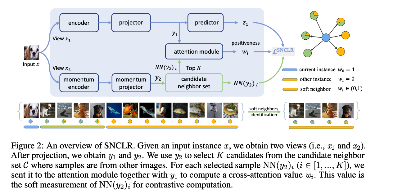
Procedure

• step 1) Given current instance \(x\) , culltivate a candidate neighbor set
  • \(\mathrm{NN}\left(y_2\right)_i(i \in[1,2, \ldots, K])\) : select \(K\) candidate
    • \(\mathrm{NN}(\cdot)\) : the nearest neighbor identification operation
• step 2) sent it to the attention module together with \(y_1\)
  • for cross-attention computations.
  • predicts a positiveness value \(w_i\).
    • use this value to adjust the contributions of \(\mathrm{NN}\left(y_2\right)_i\) to \(z_1\) in CL

Loss function :

\(\mathcal{L}_x^{\mathrm{SNCLR}}=-\frac{1}{N} \log \frac{\sum_{i=0}^K w_i \cdot \exp \left(z_1 \cdot \mathrm{NN}\left(y_2\right)_i / \tau\right)}{\sum_{i=0}^K \exp \left(z_1 \cdot \mathrm{NN}\left(y_2\right)_i / \tau\right)+\sum_{i=1}^{N-1} \sum_{j=0}^K \exp \left(z_1 \cdot \mathrm{NN}\left(y_2^{i-}\right)_j / \tau\right)}\).

Notation

• \(z_1\) :predictor output

• \(\mathrm{NN}\left(y_2\right)_0\) : \(y_2\)
• \(\mathrm{NN}\left(y_2^{i-}\right)_0\) : \(y_2^{i-}\)
• \(w_0\) : set as \(1\)
• \(\mathrm{NN}\left(y_2^{i-}\right)\) is the nearest neighbors search of each \(y_2^{i-}\) to obtain \(K\) neighbors (i.e., \(\mathrm{NN}\left(y_2^{i-}\right)_j\), \(j \in[1,2, \ldots, K])\).

Pos / Neg pairs:

• partially positive pairs : \(z_1\) and \(\mathrm{NN}\left(y_2\right)_i\)
• negative pairs : \(z_1\) and \(\mathrm{NN}\left(y_2^{i-}\right)_j\)

If we exclude the searched neighbors of \(y_2\) and \(y_2^{i-}\)… same as InfoncE

Candidate Neighbors.

( follow SwaV )

use a queue as candidate neighbor set \(\mathcal{C}\),

• each element is the projected feature representation from the momentum branch.

when using sample batches for network training,

store their projected features in \(\mathcal{C}\) and adopt FIFO strategy to update the candidate set.

• length : relatively large to sufficiently provide potential neighbors

cosine similarity : selection metric.

nearest neighbors search :

• \[\mathrm{NN}\left(y_2\right)=\underset{c \in \mathcal{C}}{\arg \max }\left(\cos \left(y_2, c\right), \operatorname{top}_{\mathrm{n}}=K\right)\]
  • where both \(y_2\) and \(c \in \mathcal{C}\) are normalized before computation.

Positiveness Predictions.

• measure the correlations of the selected \(K\) neighbors w.r.t current instance

• introduce an attention module to softly measure their correlations (= positiveness)

• contains 2 feature projection layers

  • (1) cross-attention operator

  • (2) nonlinear activation layer.

Given two inputs \(y_1\) and \(\mathrm{NN}\left(y_2\right)_i\) … the positiveness score :

\(\rightarrow\) \(w_i=\frac{1}{\gamma_i} \operatorname{Softmax}\left[f_1\left(y_1\right) \times f_2\left(\mathrm{NN}\left(y_2\right)_i\right)^{\top}\right]\)

• \(f_1(\cdot)\) and \(f_2(\cdot)\) : the projection layers of this attention module
• \(\gamma_i\) : scaling factor to adjust positiveness \(w_i\).