PatchMixer; A Patch-Mixing Architecture for Long-term Time Series Forecasting

PatchMixer: A Patch-Mixing Architecture for Long-term Time Series Forecasting (ICLR, 2024 (?))

Contents

1. Abstract

2. Introduction

3. Related Work

4. Proposed Method

5. Experiments

Abstract

Transformer vs. CNN

• Transformer: permutation-invariant \(\rightarrow\) PatchTST

• CNN: permutation-variant \(\rightarrow\) PatchMixer

PatchMixer

• only uses depthwise separable CNN

• allows to extract

  • local featurers
  • global correlations

  using a single-scale architecture

• dual forecasting heads

  • encompass both “linear & nonlinear” components

1. Introduction

Effectiveness of Transformers in LTSF…??

PatchTST = (1) Patching + (2) TST (=Transformer)

• recent works also adopt this “patching” (Zhang & Yan, 2023; Lin et al., 2023)

Contribution

• (1) propose PatchMixer, based on CNN
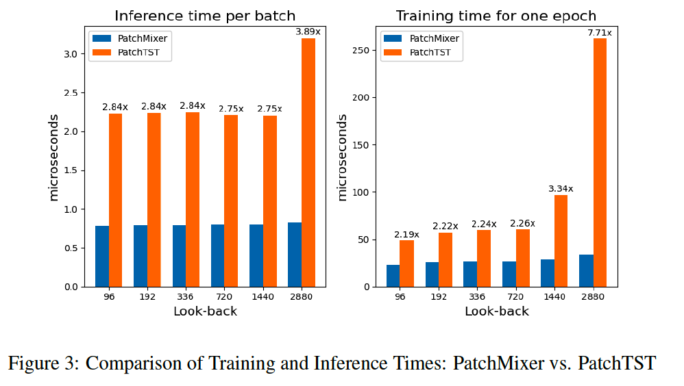
• (2) Efficient
  • 3 times faster for inference
  • 2 times faster during training
• (3) SOTA

2. Related Work

(1) CNN

TCN: dilated causal CNN

SCINet: extract multi-resolutions via binary tree structure

MICN: multi-scale hybrid decomposition & isometric convolution from both local & global perspective

TimesNet: segment sequences into patches

S4: use structured state space model

(2) Depthwise Separable Convolution

(3) Channel Independence

CI ise more effective than channel mixing methods for forecasting tasks

3. Proposed Method

(1) Problem Formulation

Look-back window \(L:\left(\boldsymbol{x}_1, \ldots, \boldsymbol{x}_L\right)\),

• \(\boldsymbol{x}_t\) : vector of \(M\) variables

Prediction sequence : \(\left(\boldsymbol{x}_{L+1}, \ldots, \boldsymbol{x}_{L+T}\right)\).

Channel Indepdendence

• Input: multivariate TS \(\left(\boldsymbol{x}_1, \ldots, \boldsymbol{x}_L\right)\) is split to \(M\) univariate TS \(\boldsymbol{x}^{(i)} \in \mathbb{R}^{1 \times L}\).
  • \(i\)-th univariate TS : \(x_{1: L}^{(i)}=\) \(\left(\boldsymbol{x}_1^{(i)}, \ldots, \boldsymbol{x}_L^{(i)}\right)\) where \(i=1, \ldots, M\).
  • independently fed into the mode
• Output: \(\hat{\boldsymbol{x}}^{(i)}=\left(\hat{\boldsymbol{x}}_{L+1}^{(i)}, \ldots, \hat{\boldsymbol{x}}_{L+T}^{(i)}\right) \in \mathbb{R}^{1 \times T}\)

(2) Model Structure

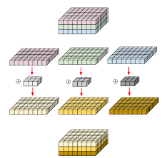
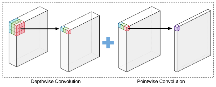
(1) (single-scale) Depthwise separable convolutional block

• to capture both the global receptive field & local positional features

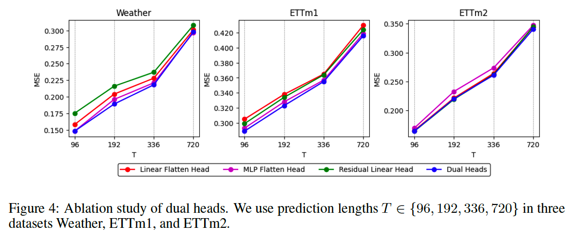
(2) Dual forecasting heads

• a) one linear flatten head and

• b) one MLP flatten head

  \(\rightarrow\) jointly incorporate nonlinear and linear features to model future sequences independently

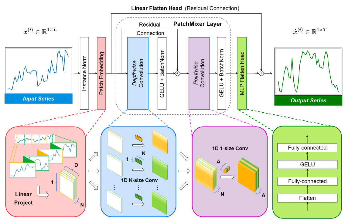
(3) Patch Embedding

( Inspired by PatchTST )

• \(\hat{\mathbf{X}}_{2 \mathrm{D}}=\operatorname{Unfold}\left(\text { ReplicationPad }\left(\mathbf{X}_{1 \mathrm{D}}\right), \text { size }=P, \text { step }=S\right)\).
• P = 16 and S = 8 ( half-overlap between each patch )

Strong predictive performance observed in TS forecasting

• Transformer (X)
• Patching (O)

\(\rightarrow\) Design PatchMixer based on CNN architectures

Embedding w/o Positional Encoding

Candidate

• a) Traditional Transformer based models

• b) PatchTST (Transformer based)

• c) PatchMixer (CNN)

a) \(\operatorname{Embedding}(\mathbf{X})=\operatorname{sum}(T F E+P E+V E): x^L \rightarrow x^D\).

b) \(\operatorname{Embedding}(\mathbf{X})=\operatorname{sum}(P E+V E): x^{N \times S} \rightarrow x^{N \times D}\)

c) \(\operatorname{Embedding}(\mathbf{X})=V E: x^{N \times S} \rightarrow x^{N \times D}\).

TFE: Temporal Feature Encoding

• ex) MinuteOfHour, HourOfDay, …

PE: Positional Embedding

VE: Value Embedding

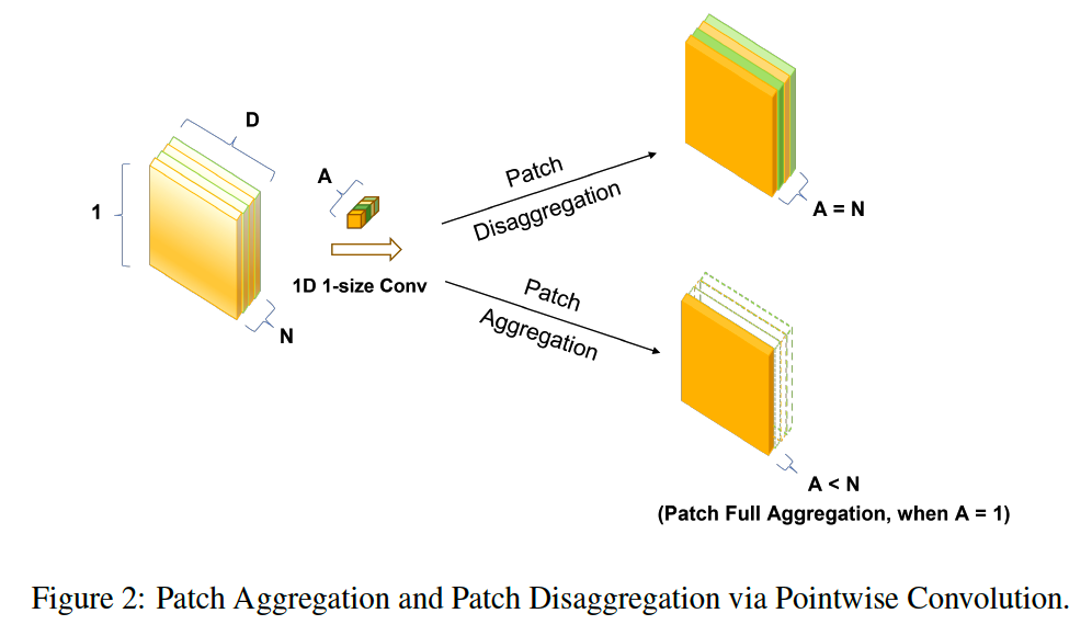
(4) PatchMixer Layer

Previous CNNs

• often modeled global relationships within TS across multiple scales or numerous branches

PatchMixer

• only employs single scale depthwise separable convolution

• patch-mixing: separates

  • per-location (intra-patch) operations with depthwise convolution
  • cross-location (inter-patch) operations with pointwise convolution

  \(\rightarrow\) allows our model to capture both the global receptive field and local positional features

(5) Dual Forecasting Heads

Previous LTSF methods

• a) decomposing inputs (i.e. DLinear)
• b) multi-head attention mechanism in Transformers: decomposing & aggregating multiple outputs.

\(\rightarrow\) prropose novel dual-head mechanism based on the decomposition-aggregation concept

Dual-head mechanism

• Capture linear features and the other focuses on capturing nonlinear variations
• extracts the …
  • (1) overall trend of temporal changes
    • via a linear residual connection spanning the convolution
  • (2) nonlinear part
    • Via an MLP forecasting head after a fully convolutional layer
• prediction results = sum of the two

(6) Normalization & Loss Function

Instance Norm

Loss function

• \(\begin{gathered} \mathcal{L}_{\mathcal{M S E}}=\frac{1}{M} \sum_{i=1}^M \mid \mid \hat{\boldsymbol{x}}_{L+1: L+T}^{(i)}-\boldsymbol{x}_{L+1: L+T}^{(i)} \mid \mid _2^2, \\ \mathcal{L}_{\mathcal{M A E}}=\frac{1}{M} \sum_{i=1}^M \mid \mid \hat{\boldsymbol{x}}_{L+1: L+T}^{(i)}-\boldsymbol{x}_{L+1: L+T}^{(i)} \mid \mid . \end{gathered}\).

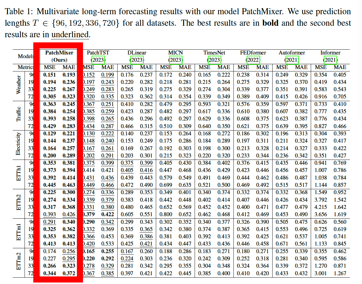
4. Experiments

(1) LTSF task

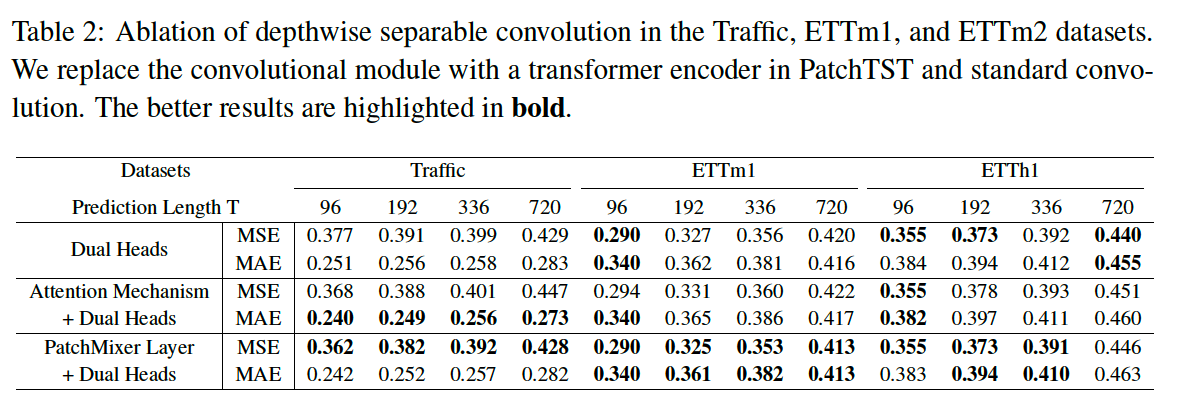
(2) Ablation Study

a) Efficiency analysis

b) Conv vs. Attention

c) Dual Forecasting head

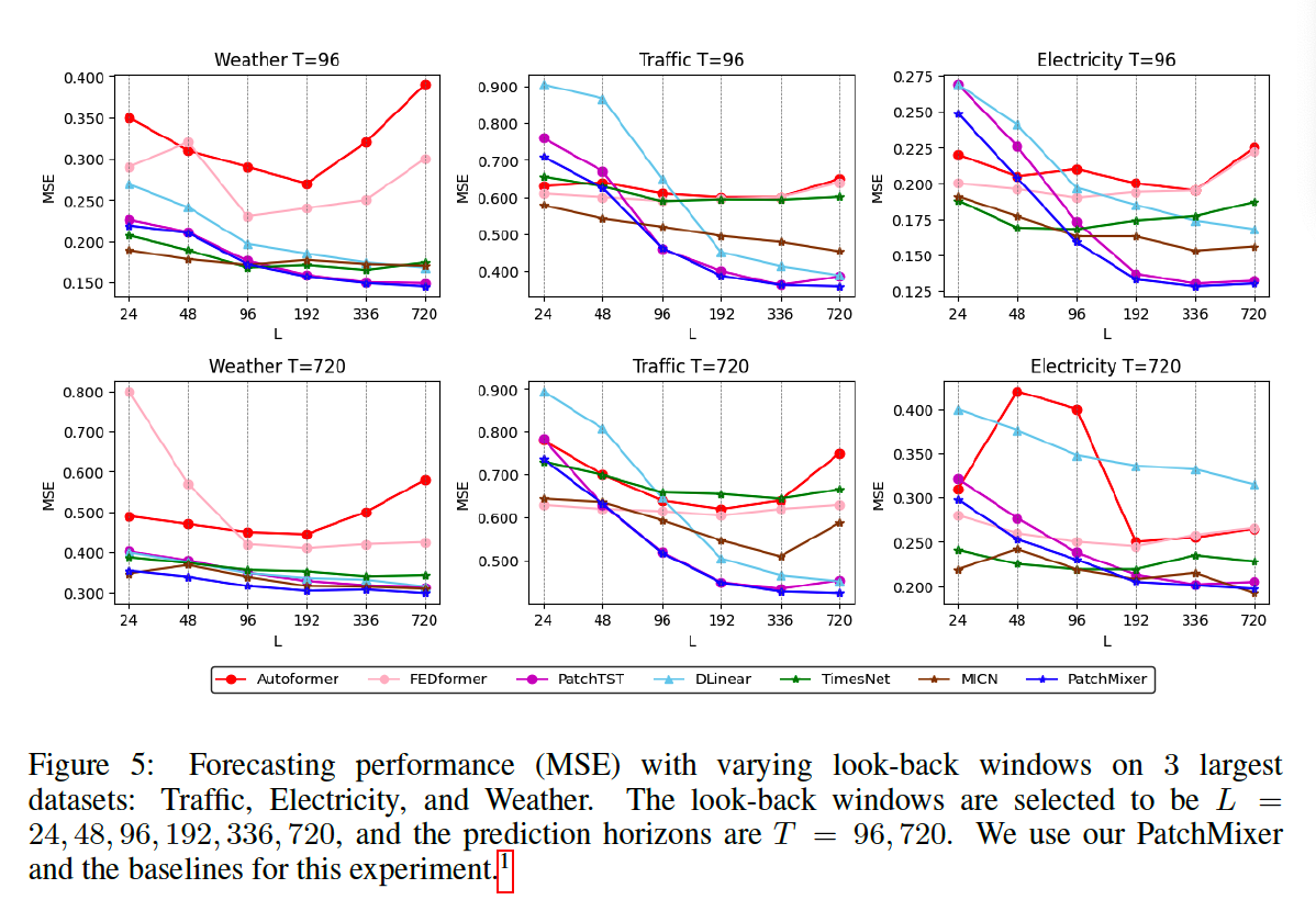
d) Varying Lookback Window