DAM; Towards a Foundation Model for Time Series Forecasting

DAM: Towards A Foundation Model for Time Series Forecasting (ICLR, 2024 (?))

Contents

1. Abstract
2. Introduction
3. Related Work
4. The DAM, explained
5. Experiments

Abstract

Universal forecating

• TS with multiple distinct domains & different underlying collection procedures

Existing methods: assume “regularity”

• (1) input data is regularly sampled
• (2) forecast pre-determined horizon

\(\rightarrow\) failure to generalize!

DAM

• Input: randomly sampled histories
• Output: adjustable basis composition ( as a continuous function of time )
  • Non-fixed horizon
• 3 components
  • (1) flexible approach for using randomly sampled histories from a long-tail distn
    • Q1) 멀리있더라도, 도움이 되는 정보가 있을 수 있지 않을까? ( = seasonality )
  • (2) transformer backbone
    • Q2) CNN, MLP는?
  • (3) basis coefficients of a continuous fujnction of a time

Experiment

Single univariate DAM trained on 25 TS datasets

• SOTA across multivariate LTSF across 18 datasets
  • 8 held-out for zero-shot
• robust to missing & irregularly sampled data

1. Introduction

Previous SOTA methods: FIXED-length common-interval sequences ( = regular TS )

\(\rightarrow\) does not scale well for many practical applications

\(\rightarrow\) we need more generaliezd forecasting methods!

Why does existing methods fail to generalize outside the scope of their training?

• (1) assume INPUT data is FIXED-length & REGULARLY sampled

  ( = evenly spaced & ordered )

• (2) assume pre-determined forecasting horizon

\(\rightarrow\) need to relax these assumptions for universal forecasting

Universal forecasting

• (1) must be robust to underlying collection processes
• (2) must be robust to cross-domain differences

DAM (Deep data-dependent Approximate analytical Model)

= foundation model for TS for universal forecasting

• (1) takes in randomly sampled histories
• (2) outputs time-function forecasts
• (3) use transformer backbone

2. Related Work

PatchTST/Dlinear/N-HiTS..

Multi-scale modeling

• (1) TimesNet & MICN
  • use multi-scale mechanism, breaking the task up into multiple scales where CNN can operate
• (2) Pyraformer & Crossformer
  • use custom hierarchical attention
• (3) LightTS
  • applies down sampling an MLP to model at multiple scales
• (4) DAM
  • use basis function composition
  • can also access the distant past due to historical sampling regime

Frequency-domain modeling

• (1) Autoformer
  • autocorrelation-based attention
• (2) Fedformer
  • frequency domain enables global perspective
  • uses frequency enhanced block & Fourier projeiction
• (3) FiLM
  • uses Legrende polynomials & Fourier projections
• (4) ETSFormer
  • uses 2 attention mechanisms that use ..
    • a) exponential decay to explicitly bias toward recent history
    • b) high amplitude fourier components
• (5) DAM
  • operates in both frequency & time domains

3. The DAM, explained

DAM = single model for multiple Ts datastes across domains

• (1) Backbone: Transformer
• (2) Input: Historical Sampling Regime (HSR)
  • ingest context data sampled from long-tail distn
• (3) Output: coefficients of basis functions
  • define the shape of a continuous function of time, \(f(t)\)

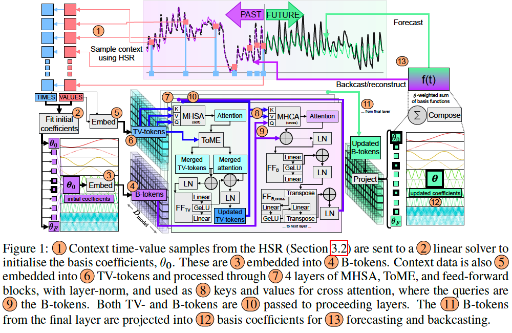
(1) Backbone

• \(D_{\text {model }}\) : latent dimension
• Input
  • (1) univariate (time-value) tuple + with time units of day
    • sampled from HSR
    • (i.e., \(\delta t=1\) is a 1 day interval),
  • (2) initialised basis coefficients + with corresponding frequency information
• Tokens
  • (1) (time-value) tuple \(\rightarrow\) TV-tokens
  • (2) initialised Basis coefficients \(\rightarrow\) B-tokens
  • (3) Affine token: initialised with 50 evenly-spaced percentiles of the values for affine adjustments.

Model Structure

4 layers of processing, where each layer consists of …

• 4 heads of multi-head self-attention (MHSA) for TV-tokens
• 4 heads of cross-attention for B-tokens
  • Q = B-tokens
  • K & V = TV-tokens
• 3 separate feed-forward blocks for
  • TV-tokens
  • Affine token
  • B-tokens
• Additional feed-forward block acting across B-tokens
• Multiple layer normalization (LN) layers
• Token merging
  • used to reduce the number of TV-tokens during each layer of processing.

Other details:

• Simple compared to earlier methods!
  • ( uses standard MHSA, not a time series-specific variant )
• Data need not be regularly sampled to yield continuous ‘blocks’
• No explicit multi-scale mechanisms are required

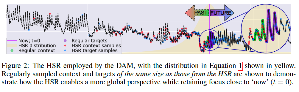
(2) Historical Sampling Regime (HSR)

Input: irregular and variable-length data

\(\rightarrow\) making it suitable to a broader variety of TS datasets & domains

\(\rightarrow\) can be trained easily on a large collection of TS datasets

( & miitigating early overfitting common in TS forecasting )

Uses a long-tail distribution over time steps

• \(x = t/R\), where \(R\) is the sample resolution (e.g., hourly)
• call this the history sampling regime (HSR)
  • \(p_{\mathrm{hsr}}(x)=\frac{1}{c} \cdot \frac{1}{1+\frac{x}{\sigma}^2}\).
    • \(c\) : normalisation constant
    • \(\mathrm{X}\) : sample support
    • \(\sigma\) : HSR ‘width’
      • smaller \(\sigma\) biases sampling recent past more than distant past.
  • used to sample \(x\), from which \((t, v)\) tuples are built, where \(v\) is the value at time \(t\).
  • used for both
    • context data from the past \((x<0)\)
    • target data (any \(x\)).
  • number of points: *variable

Figure 2

• HSR-based context : gives access to a more global perspective
• Distribution: icreases the likelihood of sampling the distant past
  • enabling a global perspective of the signal
  • still ensure that the majority of samples are recent.

(3) Basis Function Composition

Select 437 frequencies

• 1 minute (1/1440 days) ~ 10 years(52x7x10 days)
• range: minute / hour / day /week year
  • enable wide basis function coverage

Basis function composition

\(f(t, \boldsymbol{\theta}, \boldsymbol{\nu})=\operatorname{IQR}\left(a\left(\sum_{\nu=\frac{1}{1440}}^{52 \cdot 7 \cdot 10} \theta_{\nu, 1} \sin (2 \pi \nu t)+\theta_{\nu, 2} \cos (2 \pi \nu t)\right)-b\right)+M E D\).

• \(\theta\) : output vector from the DAM ( = basis function coefficients )
• \(\nu \in \mathbf{\nu}\) : frequency
• \(\theta_{\nu, 1}\) and \(\theta_{\nu, 2}\), : coefficients for sine and cosine functions at frequency \(\nu\)
• MED & IQR: Median and inter-quartile range per-datum
  • for online robust standardisation
• \(a\) & \(b\) : affine adjustments
  • also output from the DAM

Previous methods vs. DAM

• (previous) leverage basis functions that use some form of implicit basis
  • (i.e., within the model structure)
• (DAM) use explicit composition
  • 2 major advantages:
    • (1) no fixed horizon and can be assessed for any \(t\)
    • (2) basis functions are naturally interpretable

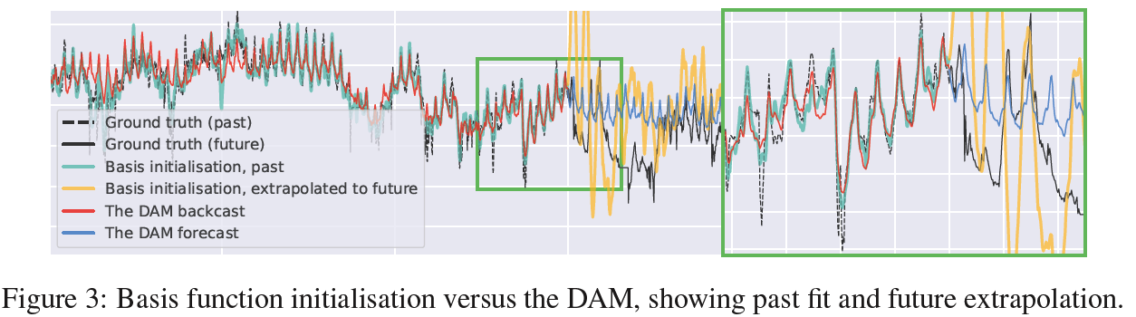
Basis function initialisation.

Advantageous to initialise B-tokens with basis coefficients fit to the context

• use a linear differential equation solver to find initialisation coefficients, \(\boldsymbol{\theta}_0\).

(4) Training

Loss function: Huber loss

• both RECONSTRUCT & FORECAST loss

Number of context points sampled from the HSR for context and targets : 540

\(\sigma\) : 720 during training

Before aggregation, the loss was re-scaled element-wise using an exponential decay of \(2^{-x / 360}\)

Train SINGLE DAM on 25 time series datasets

Iterations: 1,050,000

(5) Inference

Needs only (time-value) pairs from a given variable

Procedures

• (1) extract time-value pairs
  • using the HSR probability defined over \(x\)
  • sample indices using a weighted random choice (w/o replacement)
• (2) compute \(\boldsymbol{\theta}_0\) from context
  • \(\boldsymbol{\theta}_0\) is input to the model and not one of the model parameters
• (3) forward pass to produce \(\boldsymbol{\theta}\)
• (4) compute basis composition at \(t\) or any other query times

Adopt channel-independence

HSR tuning

Significant advantage: iits settings (context size and \(\sigma\) ) can be set after training for better forecasting.

• estimate MSE per-dataset for a range of context sizes and \(\sigma\)
  • Section 4.1 shows our results with and without this tuning

4. Experiments

33 datasets for training and evaluation

Training

• Augment 10 commonly used datasets
  • split into train/valid/test
• 15 datasets are additionally used to enhance training

Evaluation

• 10 datasets : within-dataset generalisation
  • ETTh1, h2, m1, and m2; ECL; Traffic; Weather; USWeather; Exchange; and Wind
• 8 held-out datasets : Illness, Weekdays, UCIPower, Azure, MTemp, MWeb, MWeather, and MMeters

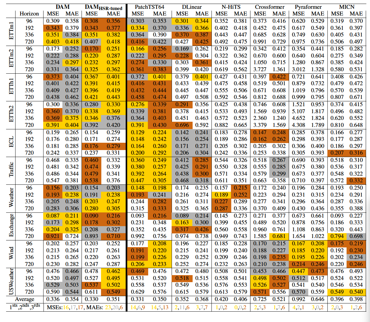
(1) Long-term TS Forecasting

• Average of 3 seeds

• 6 SOTA methods

• DAM HSR-tuned : used optimal HSR values based on validation set performance
• Baselines : specialise on dataset-horizon combinations
  • each baseline required 40 unique variants ( \(\leftrightarrow\) one model for DAM )

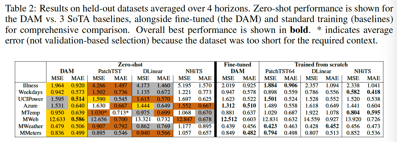
(2) Forecasting on Held Out Datasets

Foundation model

• should transfer well within scope but outside of its training datasets
• either under..
  • fine-tuning
  • zero-shot
• tested both protocols on 8 datasets held out datasets

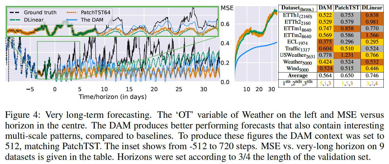
(3) VERY long-term forecasting

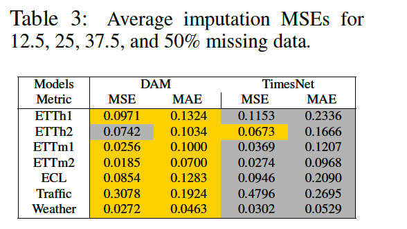
(4) Held out task: Imputation

TimesNet: SoTA on imputation task

No training of the backbone is even required in this case because the initialisation coefficients are optimal for past data.