(paper) Learning Graph Structures with Transformer for MTS Anomaly Detection in IoT

Learning Graph Structures with Transformer for MTS Anomaly Detection in IoT (2022)

Contents

1. Abstract
2. Introduction
3. Problem Statement
4. Methodology
   1. Gumbel-Softmax Sampling
   2. Influence Propagation via Graph Convolution
   3. Hierarchical Dilated Convolution
   4. More Efficient Multi-branch Transformer

0. Abstract

Detecting anomaly in MTS

• difficult, due to temporal dependency & stochasticity

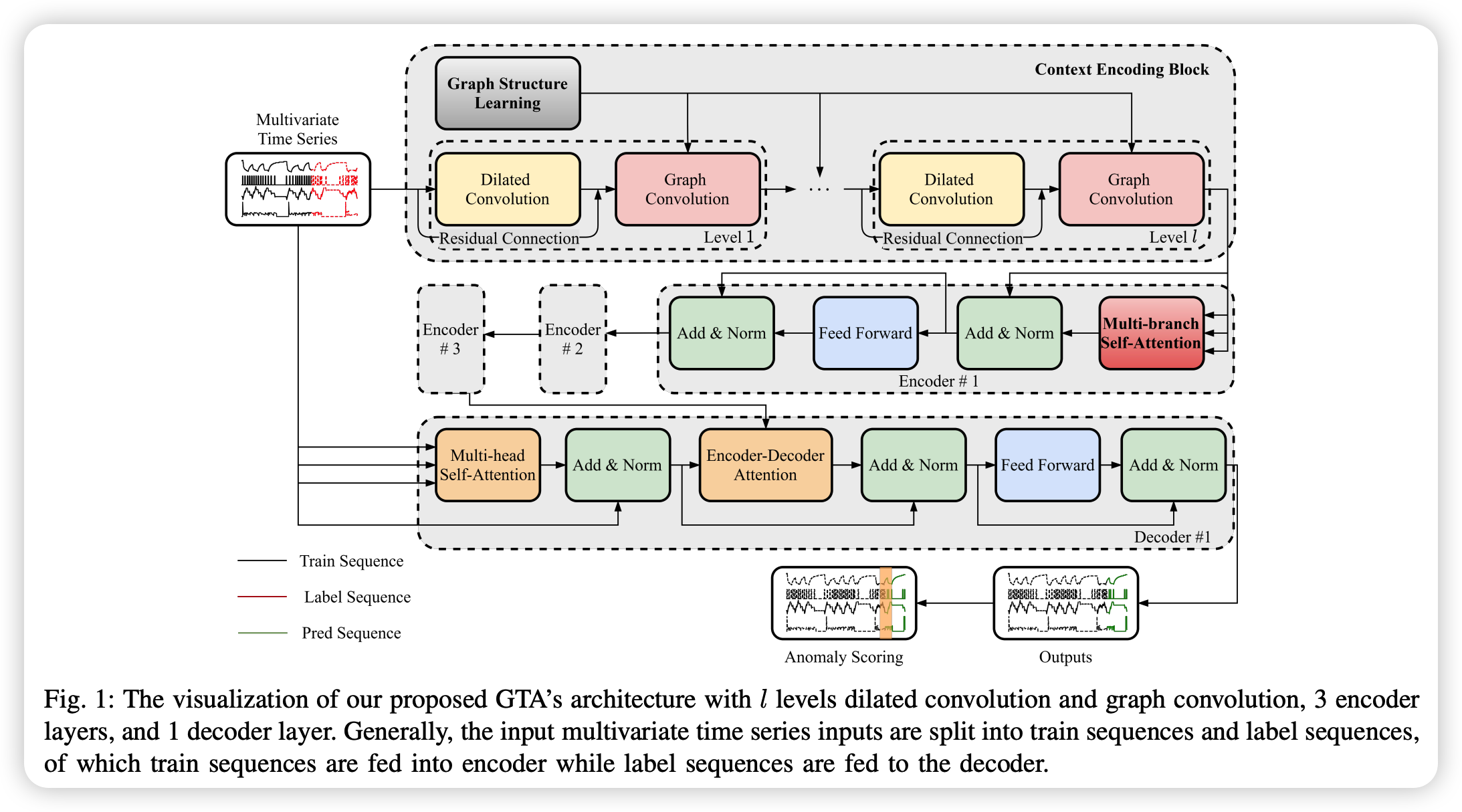
GTA

• new framework for MTS anomaly detection
• automatically learning a graph structure, graph convolution, modeling temporal dependency using Transformer
• connection learning policy
  • based on Gumbel-softmax sampling
  • learn bi-directed links among sensors
• Influence Propagation convolution
  • anomaly information flow between nodes

1. Introduction

Existing GNN approaches

• use cosine similarity to learn the graph structure
• then, define top-K closest nodes as the source nodes’ connections
• then, do GAT

Problem with previous works?

• (1) dot products among sensor embeddings lead inevitably to QUADRATIC TIME & SPACE complexity, regarding the number of sensors
• (2) the TIGHTNESS of spatial distance can not entirely indicate that there exists a string connection in a topological structure

propose GTA (Graph learning with Transformer for Anomaly detection)

• learning a global bi-directed graph
• through a connection learning policy ( based on Gumbel Softmax Sampling )
  • to overcome quadratic complexity & limitations of top-K nearest strategy

Transformer vs RNN

• Parallizeable!

Contribution

• novel & differentiable connection learning policy

• novel graph convolution ( = Information Propagation convolution ),

  to model the anomaly influence flowing process

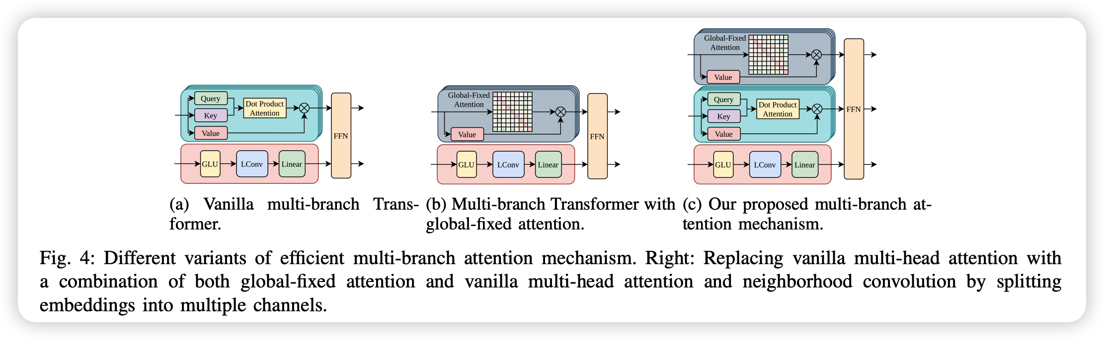
• propose a novel multi-branch attention,

  to tackle the original multi-head attention & quadratic complexity challenge

2. Problem Statement

Notation

• \(\mathcal{X}^{(t)} \in \mathbb{R}^{M}\) : MTS
  • \(M\) : total number of sensors
• \(\mathcal{X}\) : normal data
• \(\hat{\mathcal{X}}\) : data with anomalies

only construct the sequence modeling process on normal data ( without anomalies )

Forecasting-based strategy

( single-step time series forecasting )

• target : predict the time series value \(\mathbf{x}^{(t)} \in \mathbb{R}^{M}\)
• input : \(\mathbf{x}=\left\{\mathbf{x}^{(t-n)}, \cdots, \mathbf{x}^{(t-1)}\right\}\)
  • window size = \(n\)

Anomaly detection

• goal of AD : predict the output vector \(\hat{\mathbf{y}} \in \mathbb{R}^{n}\), where \(\hat{\mathbf{y}}^{(t)} \in\{0,1\}\)
• Returns an anomaly score for each testing timestamp

Definition :

• Graph : \(\mathcal{G}=(\mathcal{V}, \mathcal{E})\)
  • \(\mathcal{V}=\{1, \cdots, M\}\) : set of nodes
  • \(\mathcal{E} \subseteq \mathcal{V} \times \mathcal{V}\) : set of edges
• Node Neighborhood : \(\mathcal{N}(i)=\left\{j \in \mathcal{V} \mid \mathbf{e}_{i, j} \in \mathcal{E}\right\}\)

3. Methodology

Each sensor = specific node in the graph

• previous methods : pick top-K closest node as neighbor

• proposal : devise a directed graph structure learning policy,

  to automatically learn the adjacency matrix!

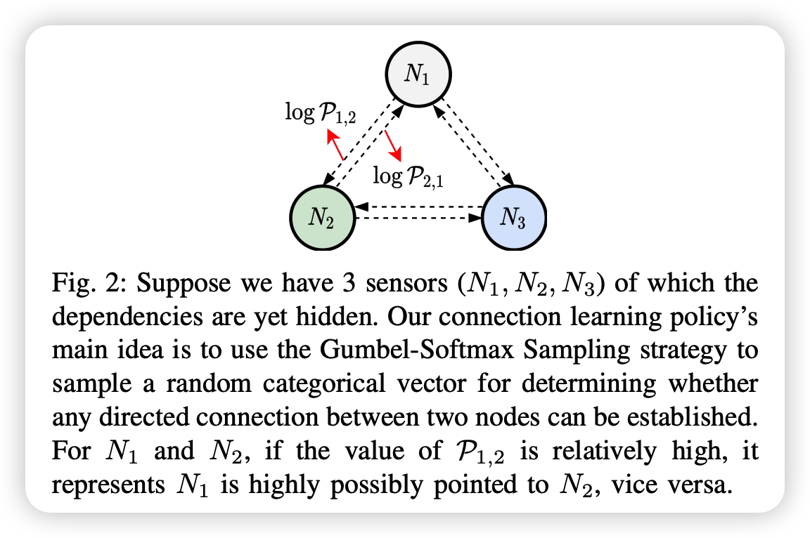
Core of learning policy = Gumbel-softmax Sampling strategy

• inspired by policy learning network in RL
• discovered hidden associations are fed into GCN

Construct a hierarchical context encoding block

(1) Gumbel-Softmax Sampling

Sampling DISCRETE data …. non-differentiable!

\(\rightarrow\) introduce Gumbel softmax distn

( = continuous distn over the simplex….approximate samples from categorical distn )

Gumbel-Max trick

Sample any pair of nodes’ connection strategy \(z^{i, j} \in\{0,1\}^{2}\), with…

• \(z^{i, j}=\underset{c \in\{0,1\}}{\arg \max }\left(\log \pi_{c}^{i, j}+g_{c}^{i, j}\right)\).
  • where \(g_{0}, g_{1}\) are i.i.d samples drawn from a standard Gumbel distribution

Gumbel-Softmax trick

Sample any pair of nodes’ connection strategy \(z^{i, j} \in\{0,1\}^{2}\), with…

• \(z_{c}^{i, j}=\frac{\exp \left(\left(\log \pi_{c}^{i, j}+g_{c}^{i, j}\right) / \tau\right)}{\sum_{v \in\{0,1\}} \exp \left(\left(\log \pi_{v}^{i, j}+g_{v}^{i, j}\right) / \tau\right)}\).
  • \(\tau\) : temperature ( control smoothness )

proposed method significantly reduces the computation complexity

• \(\mathcal{O}\left(M^{2}\right)\) to \(\mathcal{O}(1)\)
• (do not need dot product among high-dim node embeddings)

(2) Influence Propagation via Graph Convolution

GCN block

• model the influence propagation process

Anomaly detection

• occurrence of abnormalities is due to a series of chain influences,

  caused by one/several nodes being attacked

IP (Influence Propagation)

• applying a node-wise symmetric aggregationg operation \(\square\)
• updated output of IPConv at \(i\)-th node :
  • \(\mathbf{x}_{i}^{\prime}=\sum_{j \in \mathcal{N}(i)} h_{\Theta}\left(\mathbf{x}_{i} \mid \mid \mathbf{x}_{j}-\mathbf{x}_{j} \mid \mid \mathbf{x}_{j}+\mathbf{x}_{i}\right)\).
  • \(\mathbf{x}_{j}-\mathbf{x}_{i}\) : differences between nodes to explicitly model the influence propagation delay from node \(j\) to \(i\)

Training Strategy & Regularization

• propose a sparsity regularization \(\mathcal{L_s}\) to enhance the compactness of each node,

  by minimizing the log-likelihood of the probability of a connection

• \(\mathcal{L}_{s}=\sum_{1 \leq i, j \leq M, i \neq j} \log \pi_{1}^{i, j}\),

(3) Hierarchical Dilated Convolution

Dilated Conv ( via 1D-conv )

\(\rightarrow\) choosing the right kernel size is challenging!

\(\rightarrow\) Propose a hierarchical dilated convolution learning strategy( + GCN )

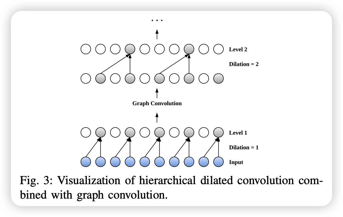
Description

• [bottom layer] MTS input ( for some time \(t\) )
• [first layer block]
  • dilated conv with dilation rate=1
• [GCN]
• [second layer block]
  • dilated conv with dilation rate=2

Able to capture LONG-term temporal dependencies

(4) More Efficient Multi-branch Transformer

(5) Overall Architecture