(paper 80) Learning Fast and Slow for Online TS Forecasting

Learning Fast and Slow for Online TS Forecasting

Contents

1. Abstract
2. Introduction
3. Preliminary & Related Work
   1. TS Settings
   2. Online TS Forecasting
   3. Continual Learning
4. Proposed Framework
   1. Online TS Forecasting as a Continual Learning Problem
   2. FSNet ( Fast and Slow Learning Networks )

0. Abstract

Data arrives sequentially.

Training deep neural forecasters on the fly is notoriously challenging

• limited ability to adapt to non-stationary environments
• fast adaptation capability of DNN is critica

Fast and Slow learning Network (FSNet)

• inspired by Complementary Learning Systems (CLS) theory
• address the challenges of online forecasting.
• improves the slowly-learned backbone
  • by dynamically balancing fast adaptation to recent changes and retrieving similar old knowledge.
• via an interaction between two novel complementary components:
  • (i) a per-layer adapter
    • to support fast learning from individual layers
  • (ii) an associative memory
    • to support remembering, updating, and recalling repeating events

1. Introduction

Batch learning setting

• whole training dataset to be made available a priori
• implies the relationship between the input and outputs remains static

Desirable to train the deep forecaster “online” (Anava et al., 2013; Liu et al., 2016)

• using only new samples to capture the changing dynamic of the environment.

• remains challenging for 2 reasons.

  • (1) Naively train DNNs on data streams REQUIRES MANY SAMPLES to converge

    • offline training benefits ( = such as mini-batches or training for multiple epochs ) are not available.
    • when a distribution shift happens, such models would require many samples

    \(\rightarrow\) DNN lack a mechanism to facilitate successful learning on data streams.

  • (2) TS often exhibit RECURRENT patterns

    • one pattern could become inactive and re-emerge in the future.
    • catastrophic forgetting : cannot retain prior knowledge

\(\rightarrow\) Consequently, online TS forecasting with deep models presents a promising yet challenging problem.

This paper

• formulate online TS forecasting as an online, task-free continual learning problem

• continual learning requires balancing two objectives:

  • (1) utilizing past knowledge to facilitate fast learning of current patterns
  • (2) maintaining and updating the already acquired knowledge

  ( = stability-plasticity dilemma )

\(\rightarrow\) develop an effective Online TS forecasting framework

• motivated by the Complementary Learning Systems (CLS)

FSNet (Fast-and-Slow learning Network)

to enhance the sample efficiency of DNN when dealing with distribution shifts or recurring concepts in online TS forecasting.

Key idea for Fast Learning

• always improve the learning at current steps

  ( = instead of explicitly detecting changes in the environment )

• employs a perlayer adapter to model the temporal consistency in TS & adjust each intermediate layer to learn better

For recurring patterns..

• equip each adapter with an associative memory
• When encountering such events, the adapter interacts with its memory to retrieve and update the previous actions to further facilitate fast learning.

Contributions

• (1) Radically formulate learning fast in online TS forecasting as a continual learning problem
• (2) Propose a fast-and-slow learning paradigm of FSNet
  • to handle both the fast changing and long-term knowledge in TS
• (3) Extensive experiments
  • with both real and synthetic datasets

2. Preliminary & Related Work

(1) TS settings

Notation

• \(\mathcal{X}=\left(\boldsymbol{x}_1, \ldots, \boldsymbol{x}_T\right) \in \mathbb{R}^{T \times n}\) : a time series of \(T\) observations, each has \(n\) dimensions.
• Input : \(\mathcal{X}_{i, e}=\) \(\left(\boldsymbol{x}_{i-e+1}, \ldots, \boldsymbol{x}_i\right)\),
• Predict : \(f_\omega\left(\mathcal{X}_{i, H}\right)=\left(\boldsymbol{x}_{i+1}, \ldots, \boldsymbol{x}_{i+H}\right)\),

(2) Online Time Series Forecasting

Sequential nature of data

No separation of training and evaluation

• Instead, learning occurs over a sequence of rounds.
  • At each round, the model receives a look-back window and predicts the forecast window.
  • Then, the true answer is revealed to improve the model’s predictions of the incoming rounds
• evaluation : accumulated errors throughout learning

Challenging sub-problems

• learning under concept drifts
• dealing with missing values because of the irregularly-sampled data

\(\rightarrow\) focus on the problem of fast learning (in terms of sample efficiency) under concept drifts

Bayesian continual learning

• to address regression problems
• However, such formulation follow the Bayesian framework, which allows for forgetting of past knowledge and does not have an explicit mechanism for fast learning
• did not focus on DNNs

(3) Continual Learning

Learn a series of tasks sequentially

( with only limited access to past experiences )

Continual learner : must achieve a good trade-off between …

• (1) maintaining the acquired knowledge of previous tasks
• (2) facilitating the learning of future tasks

Continual learning methods inspired from the CLS theory

• augments the slow, deep networks with the ability to quickly learn on data streams, either via
  • (1) Experience replay mechanism
  • (2) Explicit modeling of each of the fast and slow learning components

3. Proposed Framework

Formulates the “online TS forecasting” as a “task-free online continual learning problem”

Proposed FSNet framework.

(1) Online TS Forecasting as a Continual Learnring Problem

Locally stationary stochastic processes observation

• TS can be split into a sequence of stationary segments

  ( = Same underlying process generates samples from a stationary segment )

• Forecasting each stationary segment = Learning task for continual learning.
  • ex) split into 1 segment = no concept drifts = online learning in stationary environments
  • ex) split into more than 2 segment = Online Continual Learning
• Do not assume that the points of task switch are given!

Online, task-free continual learning formulation

Differences between our formulation vs existing studies?

a) Difference 1

• (1) Most existing task-free continual learning frameworks = IMAGE data
  • input and label spaces of images are different (continuous vs discrete)
  • image’s label changes significantly across tasks
• (2) Ours = TS data
  • input and output share the same real-valued space.
  • data changes gradually over time with no clear boundary.
  • exhibits strong temporal information among consecutive samples,

\(\rightarrow\) Simply apply existing continual learning methods to TS … BAD!

b) Difference 2

TS evolves and old patterns may not reappear exactly

\(\rightarrow\) not interested in remembering old patterns precisely, but predicting how they will evolve

\(\rightarrow\) do not need a separate test set for evaluation

( but training follows the online learning setting where a model is evaluated by its accumulated errors throughout learning )

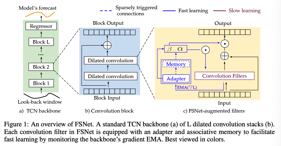
(2) FSNet ( Fast And Slow Learning Networks )

Details

• leverages past knowledge to improve the learning in the future

  ( = facilitating forward transfer in continual learning )

• remembers repeating events and continue to learn them when they reapp

  ( = preventing catastrophic forgetting )

Backbone : Temporal Convolutional Network (TCN)

• \(L\) layer with parameters \(\boldsymbol{\theta}=\left\{\boldsymbol{\theta}_l\right\}_{l=1}^L\).

Improves the TCN with 2 complementary components:

• (1) per-layer adapter \(\phi_l\)
• (2) per-layer associative memory \(\mathcal{M}_l\).

Parameters & Memories

• Total trainable parameters : \(\boldsymbol{\omega}=\left\{\boldsymbol{\theta}_l, \boldsymbol{\phi}_l\right\}_{l=1}^L\)
• Total associative memory : \(\mathcal{M}=\left\{\mathcal{M}_l\right\}_{l=1}^L\)

Notation

• \(\boldsymbol{h}_l\) : original feature map of the \(l\)-layer
• \(\tilde{\boldsymbol{h}}_l\) : adapter feature map of the \(l\)-layer

a) Fast Learning Mechanism

Key observation allowing for a fast learning?

\(\rightarrow\) facilitate the learning of each intermediate layer

Gradient EMA

\(\nabla_{\boldsymbol{\theta}_l} \ell\) : contribution of layer \(\boldsymbol{\theta}_l\) to the forecasting loss \(\ell\).

• (traditional method) move the parameters along this gradient direction

  \(\rightarrow\) results in ineffective online learning

• TS exhibits strong temporal consistency across consecutive samples

  \(\rightarrow\) EMA of \(\nabla_{\boldsymbol{\theta}_l} \ell\) can provide meaningful information about the temporal smoothness in TS

To utilize the gradient EMA …

• treat it as a context to support fast learning, via the feature-wise transformation framework

• propose to equip each layer with an adapter to map the layer’s gradient EMA to a set of smaller, more compact transformation coefficients.

• EMA of the \(l\)-layer’s partial derivative

  = \(\hat{\boldsymbol{g}}_l \leftarrow \gamma \hat{\boldsymbol{g}}_l+(1-\gamma) \boldsymbol{g}_l^t\).

  • \(\boldsymbol{g}_l^t\) : the gradient of the \(l\)-th layer at time \(t\)
  • \(\hat{\boldsymbol{g}}_l\) : the EMA.

• Adapter ( = linear layer )

  • Input : \(\hat{\boldsymbol{g}}_l\)
  • Output : Adaptation coefficients, \(\boldsymbol{u}_l=\left[\boldsymbol{\alpha}_l ; \boldsymbol{\beta}_l\right]\)

• Two-stage transformations

  • weight and bias transformation coefficients \(\boldsymbol{\alpha}_l\)
  • feature transformation coefficients \(\boldsymbol{\beta}_l\).

Adaptation process ( for layer \(\boldsymbol{\theta}_l\) )

• \(\left[\boldsymbol{\alpha}_l, \boldsymbol{\beta}_l\right]=\boldsymbol{u}_l, \text { where } \boldsymbol{u}_l=\boldsymbol{\Omega}\left(\hat{\boldsymbol{g}}_l ; \boldsymbol{\phi}_l\right)\).

• Weight adaptation: \(\tilde{\boldsymbol{\theta}}_l=\operatorname{tile}\left(\boldsymbol{\alpha}_l\right) \odot \boldsymbol{\theta}_l\)

• Feature adaptation: \(\tilde{\boldsymbol{h}}_l=\operatorname{tile}\left(\boldsymbol{\beta}_l\right) \odot \boldsymbol{h}_l\), where \(\boldsymbol{h}_l=\tilde{\boldsymbol{\theta}}_l \circledast \tilde{\boldsymbol{h}}_{l-1}\).

  • tile \(\left(\boldsymbol{\alpha}_l\right)\) : weight adaptor is applied per-channel on all filters via a tile function

    ( = repeats a vector along the new axes )

b) Remembering Recurrring Events with an Associative Memory

Old patterns may reappear

Adaptation to a pattern is represented by the coefficients \(\boldsymbol{u}\),

• useful to learn repeating events

• represents how we adapted to a particular pattern in the past

\(\rightarrow\) storing and retrieving the appropriate \(\boldsymbol{u}\) may facilitate learning the corresponding pattern when they reappear.

Associative memoy

• to store the adaptation coefficients of repeating events encountered during learning
• beside the adapter, equip each layer with an additional associative memory \(\mathcal{M}_l \in \mathbb{R}^{N \times d}\)
  • \(d\) : the dimension of \(\boldsymbol{u}_l\)
  • \(N\) : the number of elements ( fix as \(N=32\) by default.)

**Sparse Adapter-Memory Interactions **

• Interacting with the memory at every step is expensive

  \(\rightarrow\) Propose to trigger this interaction subject to a “substantial” representation change.

• Interference between the current & past representations

  = dot product between the gradients

• Deploy another gradient EMA \(\hat{\boldsymbol{g}}_l^{\prime}\) with a smaller coefficient \(\gamma^{\prime}<\gamma\)

  & Measure their cosine similarity to trigger the memory interaction as:

  • \(\text { Trigger if }: \cos \left(\hat{\boldsymbol{g}}_l, \hat{\boldsymbol{g}}_l^{\prime}\right)=\frac{\hat{\boldsymbol{g}}_l \cdot \hat{\boldsymbol{g}}_l^{\prime}}{ \mid \mid \hat{\boldsymbol{g}}_l \mid \mid \mid \mid \hat{\boldsymbol{g}}_l \mid \mid }<-\tau\).

• set \(\tau\) to a relatively high value

  = memory only remembers significant changing patterns

Adapter-Memory Interacting Mechanism

• perform the memory read and write operations using the adaptation coefficients’s EMA
• EMA of \(\boldsymbol{u}_l\) is calculated in the same manner as Equation 1.

If a memory interaction is triggered…

\(\rightarrow\) Adapter queries and retrieves the most similar transformations in the past via an attention read operation

( = which is a weighted sum over the memory items )

1. Attention calculation: \(\boldsymbol{r}_l=\operatorname{softmax}\left(\mathcal{M}_l \hat{\boldsymbol{u}}_l\right)\);
2. Top-k selection: \(\boldsymbol{r}_l^{(k)}=\operatorname{TopK}\left(\boldsymbol{r}_l\right)\);
3. Retrieval: \(\tilde{\boldsymbol{u}}_l=\sum_{i=1}^K \boldsymbol{r}_l^{(k)}[i] \mathcal{M}_l[i]\),
   • \(\boldsymbol{r}^{(k)}[i]\) : the \(i\)-th element of \(\boldsymbol{r}_l^{(k)}\)
   • \(\mathcal{M}_l[i]\) : the \(i\)-th row of \(\mathcal{M}_l\).

**Sparse attention** - by retrieving the top-k most relevant memory items ( fix as $$k=2$$. ) - The retrieved adaptation coefficient = how the model reacted to the current pattern in the past $$\rightarrow$$ combine with the current parameters as $$\boldsymbol{u}_l \leftarrow \tau \boldsymbol{u}_l+(1-\tau) \tilde{\boldsymbol{u}}_t$$, - Then we perform a **write operation** to update the knowledge stored in $$\mathcal{M}_l$$ as: $$\mathcal{M}_l \leftarrow \tau \mathcal{M}_l+(1-\tau) \hat{\boldsymbol{u}}_l \otimes \boldsymbol{r}_l^{(k)} \text { and } \mathcal{M}_l \leftarrow \frac{\mathcal{M}_l}{\max \left(1, \mid \mid \mathcal{M}_l \mid \mid _2\right)}$$.