(paper 81) A Review on Outlier, Anomaly Detection in TS data

A Review on Outlier/Anomaly Detection in TS data

Contents

1. Introduction
2. Taxonomy of Outlier Detection Techniques in the TS context
   1. Input Data
   2. Outlier Type
   3. Nature of the method
3. Point Outliers
   1. UTS
   2. MTS
4. Sequence Outliers

1. Introduction

Two types of outliers in UTS

• (1) type 1 : affects a single observation
• (2) type 2 : affects both a particular observation and the subsequent observations.

\(\rightarrow\) Extended to 4 outlier types & to the case of MTS

Many definitions of the term outlier. However still no consensus on the terms

• ex) outlier observations = anomalies, discordant observations, discords, exceptions, aberrations, surprises, peculiarities or contaminants.

Classical Definition

“An observation which deviates so much from other observations as to arouse suspicions that it was generated by a different mechanism.”

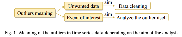
Outliers in TS can have 2 different meanings ( based on the interest of the analyst )

( Recent years ) aim to detect & analyze unusual but interesting phenomena.

• ex) Fraud detection => main objective is to detect and analyze the outlier itself.

  \(\rightarrow\) often referred to as anomalies

Section Intro

• Section 2 ) taxonomy for the classification of outlier detection techniques in TS
• Section 3 ~ 5 ) different techniques used for point, subsequence, and time series outlier detection

2. Taxonomy of Outlier Detection Techniques in the TS context

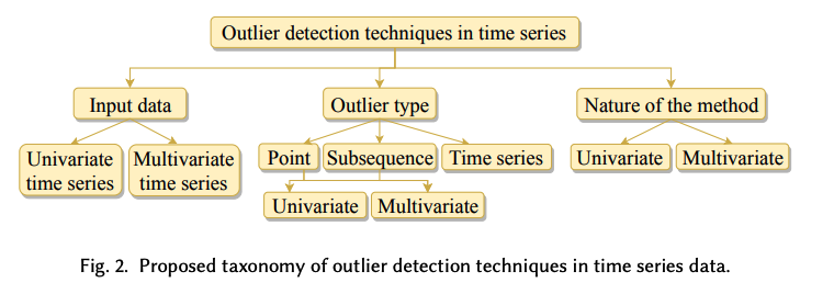
Outlier detection techniques

• vary depending on the (1) input data type, the (2) outlier type, and the (3) nature of the method

(1) Input Data

1. UTS : \(X=\left\{x_t\right\}_{t \in T}\)
   • recorded at a specific time \(t \in T \subseteq \mathbb{Z}^{+}\).
   • \(x_t\) : point or observation collected at time \(t\)
   • \(S=x_p, x_{p+1}, \ldots, x_{p+n-1}\) : subsequence of length \(n \leq \mid T \mid\)
   • assumed that \(x_t\) is a realized value of a certain r.v \(X_t\).

1. MTS : \(\boldsymbol{X}=\left\{\boldsymbol{x}_t\right\}_{t \in T}\)

• ordered set of \(k\) dim-vectors
• recorded at a specific time \(t \in T \subseteq \mathbb{Z}^{+}\)

• consists of \(k\) real-valued observations, \(\boldsymbol{x}_t=\left(x_{1 t}, \ldots, x_{k t}\right)^1\)

• \(S=x_p, x_{p+1}, \ldots, x_{p+n-1}\) : subsequence of length \(n \leq \mid T \mid\) of \(X\),
• \(X_t=\left(X_{1 t}, \ldots, X_{k t}\right)\).

(2) Outlier Type

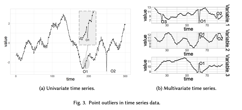
1. Point outliers.

   • behaves unusually in a specific time instant, when compared either …
     • (1) to the other values in the time series (global outlier)
     • (2) to its neighboring points (local outlier).
   • can be univariate or multivariate
     • depending on whether they affect one or more time-dependent variables
   • example) Fig 3a

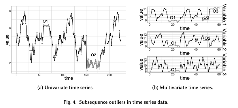
1. Subsequence outliers.
   • consecutive points in time
   • joint behavior is unusual ( although each observation individually is not necessarily a point outlier )
   • can also be global or local
   • can affect one (univariate subsequence outlier) or more (multivariate subsequence outlier) time-dependent variables

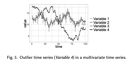
1. Outlier Time Series

• Entire time series can also be outliers

Summary

• closely related to the input data type

  • ex) If the method only allows UTS as input, then no multivariate point or subsequence outliers can be identified.

• outlier time series can only be found in MTS

• outliers depend on the context

  • ex) If the detection method uses the entire TS as contextual information

    \(\rightarrow\) then the detected outliers are global.

  • ex) If the method only uses a segment of the series (a time window)

    \(\rightarrow\) then the detected outliers are local

    ( because they are outliers within their neighborhood )

• global outliers are also local, but not all local outliers are global. (e.g., O1 in Fig. 3a).

(3) Nature of the method

Nature of the detection method employed

Univariate detection method

• only considers a single time-dependent variable

Multivariate detection method

• able to simultaneously work with more than one time-dependent variable.

Detection method can be univariate, even if the input data is MTS

( = individual analysis can be performed on each time-dependent variable )

Multivariate technique cannot be used if the input data is UTS

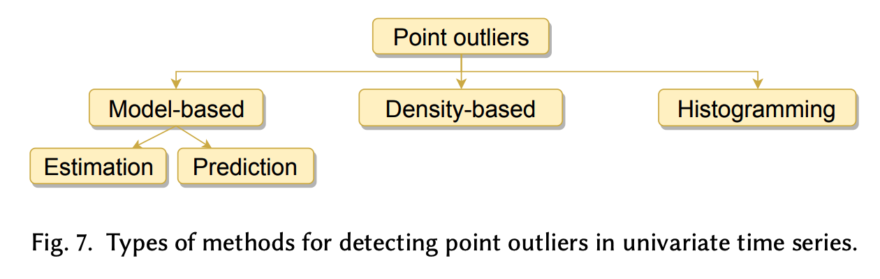
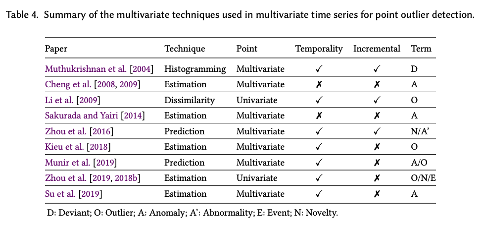
3. Point Outliers

Both in UTS & MTS

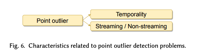
2 key characteristics

• Temporality
  • whether it considers the inherent temporal order of the observations
    • (O) produce the different results if they are applied to a shuffled version of TS
    • (X) produce the same results if they are applied to a shuffled version of TS
• Streaming & Non-streaming
  • ability to detect outliers in streaming TS ( = without having to wait for more data )

(1) UTS

detect point outliers in a UTS

• single time-dependent variable
• outliers = univariate points
• Only univariate detection techniques can be used

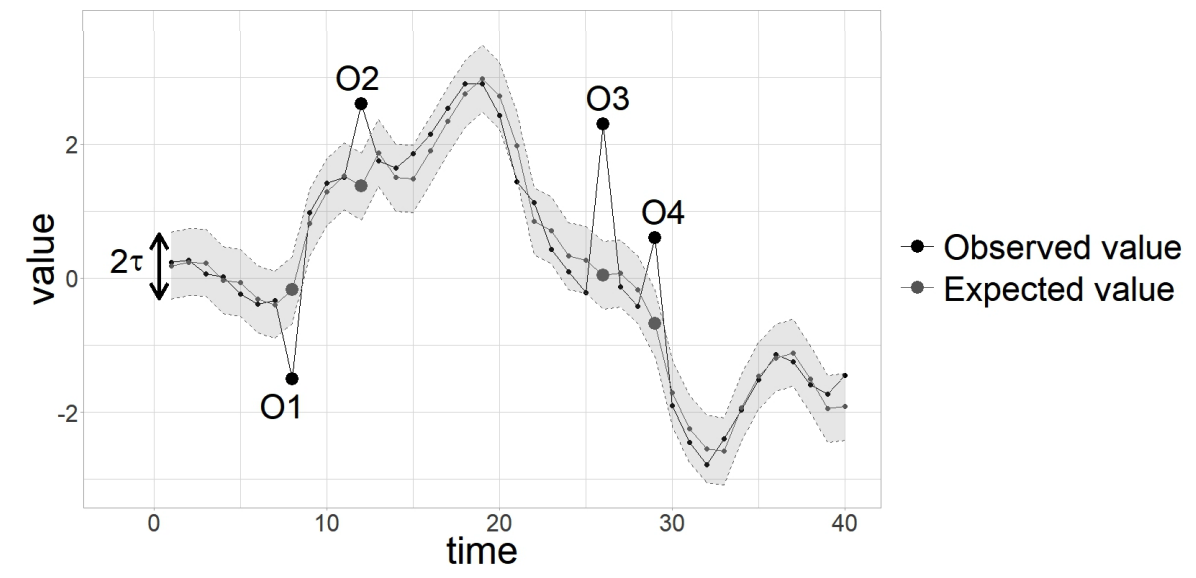
Point Outlier = point that significantly deviates from its expectve value

\(\mid x_t-\hat{x}_t \mid >\tau\).

• \(x_t\) : observed
• \(\hat{x}_t\) : expected

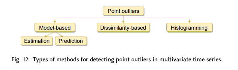
1-a) Model-based methods

• \(\mid x_t-\hat{x}_t \mid >\tau\).
• most common approaches
  • each technique computes \(\hat{x}_t\) and \(\tau\) differently
  • common ) based on fitting a model (either explicitly or implicitly).

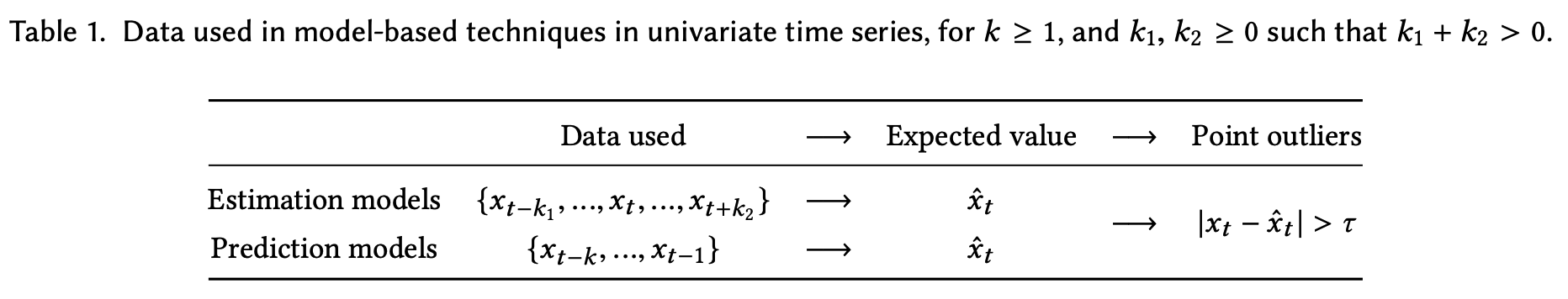
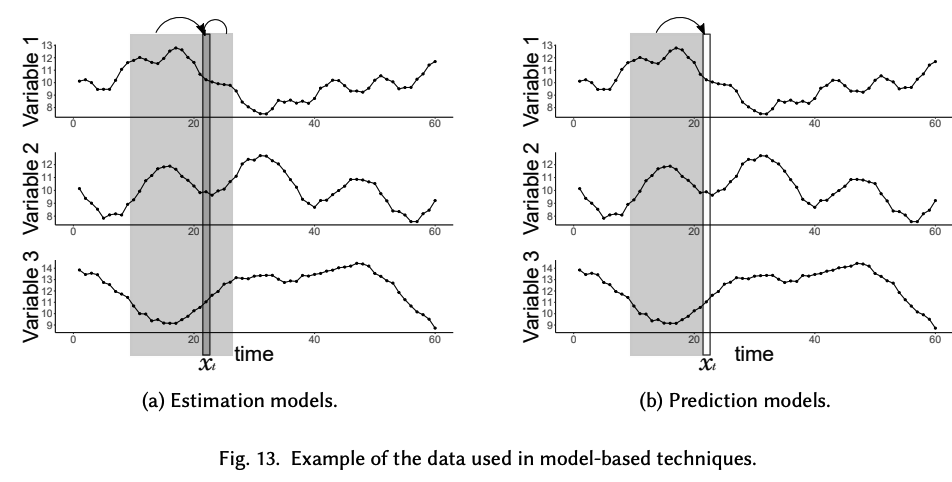
(1) Estimation model-based methods

• \(\hat{x}_t\) is obtained using previous and subsequent observations to \(x_t\) (past, current, and future data)

(2) Prediction model-based methods

• \(\hat{x}_t\) is obtained relying only on previous observations to \(x_t\) (past data)

Main difference ?

• Prediction methods : can be used in streaming TS
  • can determine whether or not a new datum is an outlier as soon as it arrives.
• Estimation methods :
  • can only be done if, in addition to some points preceding / current point \(x_t\) is used to compute

Example) Estimation based

Example 1) constant or piecewise constant models

• use basic statistics ( ex. median, Median Absolute Deviation (MAD) ) to obtain \(\hat{x_t}\)
• calculated using the full TS or by grouping the TSin equal-length segments
• cannot be applied in streaming when future data is needed (k2 > 0).

Example 2) unequal-length segments

• obtained with a segmentation technique
• ex) use the mean of each segment to determine the expected value
• ex) adaptive threshold \(\tau_i=\alpha \sigma_i\)
  • \(\alpha\) : fixed value
  • \(\sigma_i\) : std of segment \(i\)
  • \(\alpha\) is a fixed value and \(\sigma_i\) the standard deviation of segment \(i\).

Example 3)

• identify data points that are unlikely if a certain fitted model or distribution is assumed to have generated the data
• ex) model the structure of the data
  • smoothing methods ( B-splines, kernels, Exponentially Weighted Moving Average (EWMA) )
  • slope constraints
  • assume that the data are approximately normal
  • Gaussian Mixture Models (GMM).
• Once a model or distribution is assumed, use equation (1) directly to decid

Example) Prediction based

• fit a model to the TS & obtain \(\hat{x_t}\) using only PAST data

• deal with streaming TS

(A) Do not adapt to change

( = use a fixed model & not able to adapt to the changes that occur over time )

• ex) DeepAnT

  • deep learning-based outlier detection approach (CNN)

• ex) Autoregressive model / ARIMA model

  • obtain confidence intervals for the predictions instead of only point estimates.

  \(\rightarrow\) implicitly define \(\tau\)

(B) Adapt to change

( = by retraining the model )

• ex) predicts the value \(\hat{x_t}\) with the median of its past data
• ex) fit an ARIMA model within a sliding window
  • to compute the prediction interval
  • parameters are refitted each time that the window moves

Extreme Value Theory ( EVT )

• prediction-based approach
• streaming UTS
• using past data and retraining.

Details of EVT

• given a fixed risk \(q\), allows us to obtain a threshold value \(z_{q, t}\) that adapts itself to the evolution of the data

  • such that \(P\left(X_t>z_{q, t}\right)<q\), for any \(t \geq 0\),
  • assuming that the extreme values follow a Generalized Pareto Distribution (GPD).

• Data is used to both..

  • (1) detect anomalies \(\left(X_t>z_{q, t}\right)\)
  • (2) refine \(z_{q, t}\).

• example)

  • SPOT : for data following any stationary distribution
  • DSPOT : for data that can be subject to concept drift

• retrain the underlying model periodically ( or each time a new point arrives )

  \(\rightarrow\) can adapt to the evolution of TS

All of these techniques are based on \(\mid x_t-\hat{x}_t \mid >\tau\)

• but not all the existing point outlier detection methods rely on that idea

  • ex) density-based methods ( \(\leftrightarrow\) model-based methods )

    • consider that points with less than \(\tau\) neighbors are outliers

      ( \(x_t\) is an outlier \(\Longleftrightarrow \mid \left\{x \in X \mid d\left(x, x_t\right) \leq R\right\} \mid <\tau\))

1-b) Density-based methods

\(x_t \text { is an outlier } \Longleftrightarrow \mid \left\{x \in X \mid d\left(x, x_t\right) \leq R\right\} \mid <\tau\).

• \(d\) : (commonly) Euclidean distance
• \(x_t\) : data point at \(t\) step to be analyzed

Point is an outlier if \(\tau_p+\tau_s<\tau\),

• \(\tau_p\) and \(\tau_s\) are the number of preceding and succeeding neighbors at distance lower or equal than \(R\)

Widely handled in non-temporal data

• concept of neighborhood is more complex in TS due to the order
• ex) apply this method within a sliding window

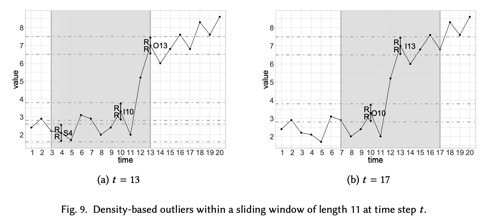
Two different time steps with \(R=0.5\), \(\tau=3\), and a sliding window of length 11.

• outlier for a window (e.g., O13 at \(t=13\) )

• NOT outlier for window (e.g., I13 at \(t=17\) )

• if a data point has at least \(\tau\) succeeding neighbors within a window…

  \(\rightarrow\) cannot be an outlier for any future evolution (e.g., S4 at \(t=13\) ).

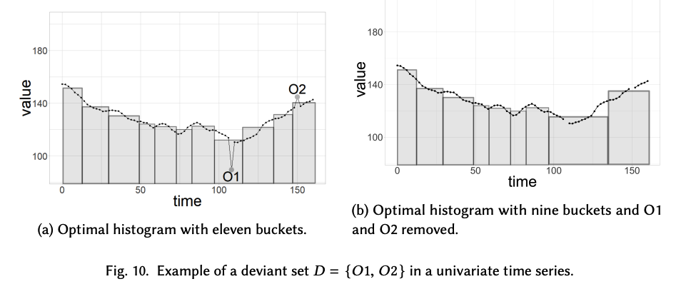
1-c) Histogramming

Detecting the points whose removal from the UTS results in a histogram representation with lower error than the original

(2) MTS

Can deal

• not only with a single variable ( 3.2.1 )
• but also with multiple variables ( 3.2.2 )

Point outlier in a MTS

\(\rightarrow\) can affect both univariate / multivariate point

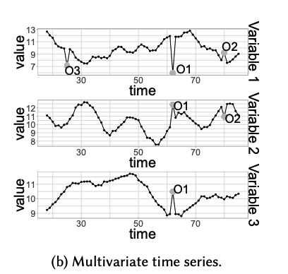
Some multivariate techniques

\(\rightarrow\) able to detect univariate point outliers

Some univariate techniques

\(\rightarrow\) able to detect multivariate point outliers

2-a) Univariate techniques.

Univariate analysis can be performed for each variable in MTS

( w/o considering dependencies that may exist between the variables )

ex) Hundman et al. [2018] : LSTM

• predict spacecraft telemetry and find point outliers within each variable in MTS
• present a dynamic thresholding approach
  • some smoothed residuals of the model obtained from past data are used to determine the threshold at each time step.

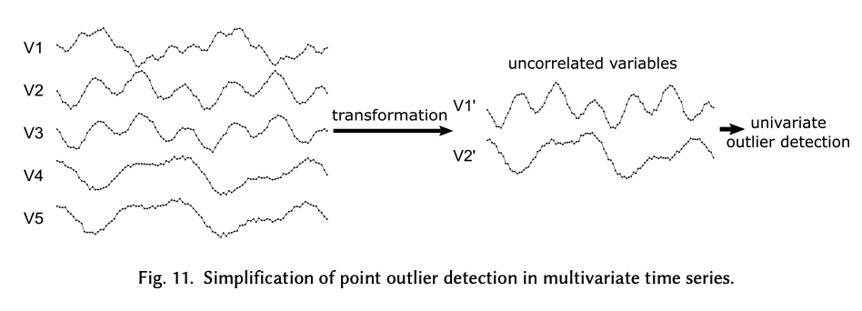
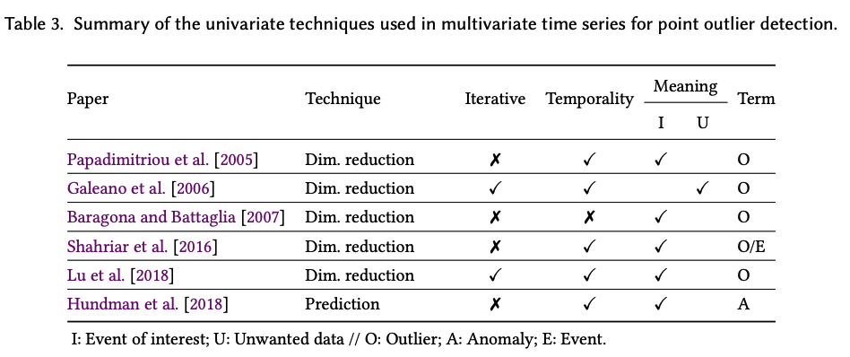
ex 2) Dimension Reduction

UTS analysis ignore correlation between TS

\(\rightarrow\) some researchers apply a preprocessing method to the MTS to find a new set of uncorrelated variables where univariate techniques can be applied.

• based on dimensionality reduction techniques,

• ex) incremental PCA ( Papadimitriou et al. [2005] )
  • linear combinations of the initial variables
  • to determine the new independent variables
  • posterior univariate point outlier detection technique that is applied is based on the AR model
• ex) Reducing the dimensionality with projection pursuit ( Galeano et al. [2006] )
  • aims to find the best projections to identify outliers.
  • prove that the optimal directions = those that maximize or minimize the kurtosis coefficient of the projected TS
  • Univariate statistical tests [Chen and Liu 1993; Fox 1972] are then applied iteratively to each projected TS
• ex) ICA ( Baragona and Battaglia [2007] )
  • to obtain a set of unobservable independent nonGaussian variables
    • assumtion : observed data has been generated by a linear combination of those variables

ex 3) Dimension Reduction 2

• reduce the input MTS into a single time-dependent variable

  ( rather than into a set of uncorrelated variables )

• ex) Lu et al. [2018]

  • define the transformed UTS using the cross-correlation function between adjacent vectors in time

  • point outliers are iteratively identified in this new TS

    ( = those that have a low correlation with their adjacent multivariate points )

2-b) Multivariate techniques

Deal simultaneously with multiple time-dependent variables ( w.o transformation )

For a predefined threshold \(\tau\), outliers are identified if

• \(\mid \mid \boldsymbol{x}_t-\hat{\boldsymbol{x}}_t \mid \mid >\tau\).
  • \(\boldsymbol{x}_t\) : actual \(k\)-dimensional data point
  • \(\hat{\boldsymbol{x}}_t\) : expected value
• \(\hat{\boldsymbol{x}}_{\boldsymbol{t}}\) can be obtained using …
  • (1) estimation models
  • (2) prediction models

Estimation model-based

Autoencoder (AE)

• outliers = non-representative features

  \(\rightarrow\) AE fails to reconstruct them

• ex) Sakurada and Yairi [2014]

  • Input = single MTS point
  • Temporal correlation between the observations within each variable is not considered

• ex) Kieu et al. [2018]

  • propose extracting features within overlapping sliding windows before applying AE

    (e.g., statistical features or the difference between the Euclidean norms of two consecutive time windows)

• ex) Su et al. [2019]

  • based on VAE & GRU
  • Input = sequence of observations containing \(\boldsymbol{x}_t\) and \(l\) preceding observations
  • Output = reconstructed \(\boldsymbol{x}_t\left(=\hat{\boldsymbol{x}}_t\right)\).
  • Apply extreme value theory in the reference of normality to automatically select the threshold value.

General trend estimation of multiple co-evolving time series

• ex) Zhou et al. [2019, 2018b]

  • non-parametric model that considers both

    • (1) temporal correlation between the values within each variable
    • (2) inter-series relatedness

    to estimate that trend.

  • Trend of each variable = estimated using MTS

  • UTS point outliers = identified within each variable

    ( instead of \(k\)-dim points )

Prediction model-based

• Fit a model to a MTS
• ex) Contextual Hidden Markov Model (CHMM)
  • incrementally captures both
    • (1) temporal dependencies :
      • modeled by a basic HMM
    • (2) correlations between the variables in a MTS :
      • included into the model by adding an extra layer to the HMM network
• ex) DeepAnt algorithm [Munir et al. 2019]
  • capable of detecting point outliers in MTS using the CNN
  • next timestamp is predicted using a window of previous observations

Dissimilarity-based methods

Based on computing the pairwise dissimilarity between MTS points

( w.o fitting the model )

For a predefined threshold \(\tau, \boldsymbol{x}_{\boldsymbol{t}}\) is a point outlier if:

• \(s\left(\boldsymbol{x}_{\boldsymbol{t}}, \hat{\boldsymbol{x}}_{\boldsymbol{t}}\right)>\tau\).

Do not usually use the raw data directly,

( instead use different representation methods )

• ex) Cheng et al. [2008, 2009]
  • represent the data using a graph
    • nodes = points in MTS
    • edges = similarity between them ( = computed with the RBF )
  • apply a random walk model in the graph
    • outlier = hardly accessible in the graph)
• ex) Li et al. [2009]
  • propose recording the historical similarity and dissimilarity values between the variables in a vector.
  • analyze the dissimilarity of consecutive points over time

Histogramming approach

pass

Summary

4. Subsequence Outliers

Goal : identify a set of consecutive points that jointly behave unusually

Key aspects

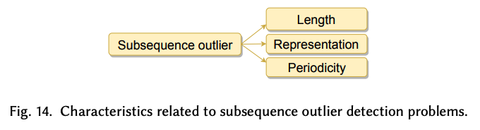
(1) Fixed-length ( \(\leftrightarrow\) variable length ) subsequences

• need the user to predefine the length
• ( commonly ) obtain the subsequences using a sliding window over TS

(2) Representation

• comparison between subsequences is challenging
• rather than raw value, use representations
  • ex) Discretization
    • equal-frequency binning, equal-width binning
  • ex) Dictionaries
    • directly to obtain representations based on dictionaries

(3) Periodicity

Periodic subsequence outliers

• are unusual subsequences that repeat over time
• Unlike point outliers where periodicity is not relevant, periodic subsequence outliers are important in areas such as fraud detection

Subsequences consider the temporality by default!

When analyzing subsequence outliers in a streaming context… 3 cases

• (1) a single data point arrives
  • answer must be given for a subsequence containing this new point
• (2) a subsequence arrives
  • needs to be marked as an outlier or non-outlier
• (3) a batch of data arrives and subsequence outliers need to be found within it

Most of the models are fixed & do not adapt to changes in the streaming sequence

\(\rightarrow\) focus on the incremental techniques!

( = more suitable for processing streaming TS )

(1) UTS

1-a) Discord detection

Comparing each subsequence with the others

\(D\) is a discord of time series \(X\) if

• \(\forall S \in A, \min _{D^{\prime} \in A, D \cap D^{\prime}=\emptyset}\left(d\left(D, D^{\prime}\right)\right)>\min _{S^{\prime} \in A, S \cap S^{\prime}=\emptyset}\left(d\left(S, S^{\prime}\right)\right)\).
  • \(A\) : set of all subsequences of \(X\) extracted by a sliding window
  • \(D^{\prime}\) : subsequence in \(A\) that does not overlap with \(D\)
    • \(S^{\prime}\) in \(A\) does not overlap with \(S\)
  • \(d\) : Euclidean distance

Discord discovery techniques require the user to specify the length of the discord.

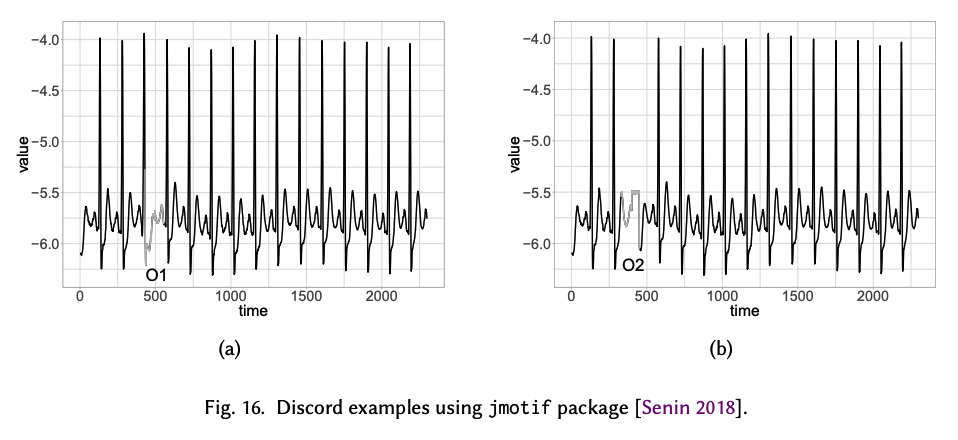
Simplest Way : Brute-force

• requires a quadratic pairwise comparison
• speed up by HOT-SAX algorithm

Limited to finding the most unusual subsequence within a TS

Problem : do not have a reference of normality or a threshold

• cannot specify whether it is indeed an outlier or not

\(\rightarrow\) Decision must be made by the user.

1-b) Dissimilarity-based methods

based on the direct comparison of subsequences, using a reference of normality

\(\rightarrow\) reference of normality vary widely

( in contrast to the dissimilarity-based techniques analyzed MTS + point outliers )

For a predefined threshold \(\tau\) , subsequence outliers are those that are dissimilar to normal subsequences

• \(s(S, \hat{S})>\tau\).

  • \(S\) : the subsequence being analyzed

  • \(\hat{S}\) : expected value of \(S\)

    ( = obtained based on the reference of normality )

• Typically, \(S\) is of fixed-length, non-periodic, and extracted via a sliding window

How to obtain \(\hat{S}\) ?

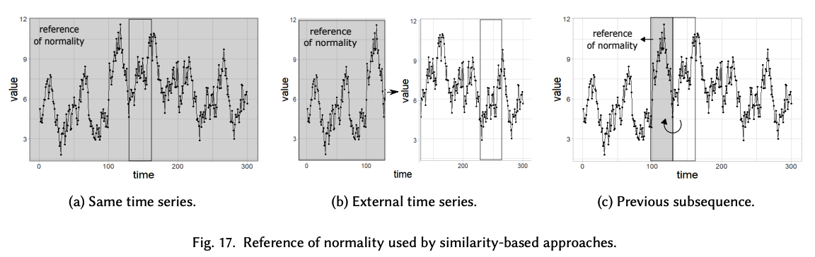
(A) same TS

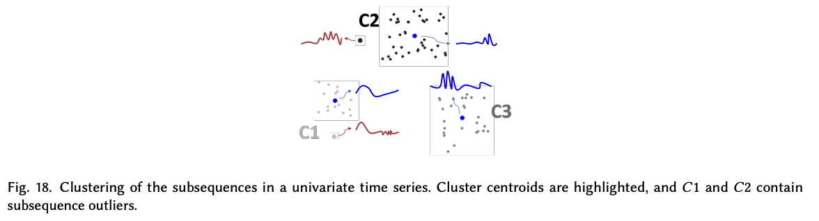
Clustering techniques

• commonly use this reference of normality to create clusters

• \(s(S, \hat{S})>\tau\). can be defined by the centroid of the cluster

  

(B) external TS

Rely on an external TS as a reference of normality

\(\rightarrow\) assuming that it has been generated by the same underlying process but with no outliers.

(C) previous subsequence

only use the previous adjacent non-overlapping window to the subsequence being analyzed as the reference of normality,

\(\rightarrow\) have a much more local perspective than the others

1-c) Prediction-based methods

Assume that normality is reflected by a time series composed of past subsequences.

• \(\sum_{i=p}^{p+n-1} \mid x_i-\hat{x}_i \mid>\tau\).
  • \(S=x_p, \ldots, x_{p+n-1}\) : subsequence being analyzed
  • \(\hat{S}\) : its predicted value

Predictions can be made in 2 different manners:

• (1) point-wise
  • make predictions for as many points as the length of the subsequence iteratively
  • errors accumulate
• (2) subsequence-wise
  • calculates predictions for whole subsequences at once (not iteratively)
  • ex) use CNN

1-d) Frequency-based methods

A subsequence \(S\) is an outlier if it does not appear as frequently as expected:

• \(\mid f(S)-\hat{f}(S)\mid >\tau\).
  • \(f(S)\) : frequency of occurrence of \(S\)
  • \(\hat{f}(S)\) : its expected frequency

Due to the difficulty of finding two exact real-valued subsequences in a TS when counting the frequencies

\(\rightarrow\) work with a discretized time series.

1-e) Information-based methods

A paradigmatic example can be found in Keogh et al. [2002]. Given an external univariate time series as reference, a subsequence extracted via a sliding window in a new univariate time series is an outlier relative to that reference if the frequency of its occurrence in the new series is very different to that expected. Rasheed and Alhajj [2014] also

https://arxiv.org/pdf/2002.04236.pdf