TimeGPT-1

TimeGPT-1

Contents

1. Abstract
2. Background
3. Foundation model for TS
4. TimeGPT
5. Experimental Results

Abstract

TimeGPT

• First foundation model for TS
• Accurate predictions for diverse datasets not seen during training
• TimeGPT zero-shot inference excels in performance, efficiency, and simplicity

1. Background

Superior capabilities of DL models are undeniable for NLP & CV…

However, TS analysis field remains skeptical of the performance of neural forecasting methods.

Why??

• (1) Misaligned or poorly defined evaluation settings
  • publicly available datasets for TS do not possess the necessary scale and volume
• (2) Suboptimal models
  • given the limited and specific datasets, even well-conceived DL architectures might struggle with generalization

TimeGPT

Larger and more diverse datasets enable more sophisticated models to perform better across various tasks.

\(\rightarrow\) TimeGPT = first foundation model that consistently outperforms alternatives with minimal complexity.

2. Foundation model for TS

Foundation models

• Rely on their capabilities to generalize across domains

  ( particularly in new datasets that were not available during training )

Forecasting model: \(f_\theta: \mathcal{X} \mapsto \mathcal{Y}\),

• \(\mathcal{X}=\left\{\mathbf{y}_{[0: t]}, \mathbf{x}_{[0: t+h]}\right\}\) and \(\mathcal{Y}=\left\{\mathbf{y}_{[t+1: t+h]}\right\}\),
  • \(h\) : forecast horizon
  • \(\mathbf{y}\) : target time series
  • \(\mathbf{x}\) : exogenous covariates

Forecasting task objective

• estimate the following conditional distribution:

  \(\mathbb{P}\left(\mathbf{y}_{[t+1: t+h]} \mid \mathbf{y}_{[0: t]}, \mathbf{x}_{[0: t+h]}\right)=f_\theta\left(\mathbf{y}_{[0: t]}, \mathbf{x}_{[0: t+h]}\right)\).

Transfer-learning

• pre-training a model on a large source dataset \(D_s=\) \(\{(\mathbf{X}, \mathbf{y}) \mid \mathbf{X} \in \mathcal{X}, \mathbf{y} \in \mathcal{Y}\}\),
• to improve its performance on a new forecasting task with target dataset \(D_t\).

2 cases of transfer learning

• (1) zero-shot learning
• (2) fine-tuning

The core idea of the presented foundation model is to leverage these principles by training it on the largest publicly available time series dataset

3. TimeGPT

(1) Architecture

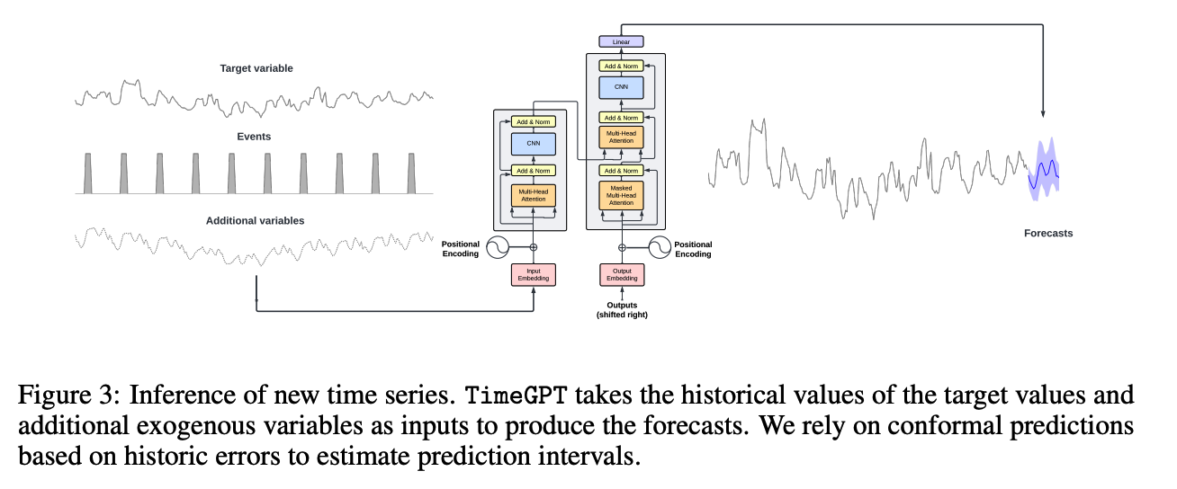
TimeGPT

• Transformer-based TS model with self-attention mechanisms
• Procedures
  • step 1) Takes a wisdow of historical values to produce the forecast
  • step 2) Adding local positional encoding
  • step 3) Maps the decoder’s output to the forecasting window dimension

Challenges of TS foundation models

• Primarily due to the complex task of handling signals derived from a broad set of underlying processes
  • ex) frequency, sparsity, trend, seasonality, stationarity, and heteroscedasticity …
• Thus, must possess the ability to manage such heterogeneity

TimeGPT

• Process TS of varied frequencies and characteristics

• Accommodate different input sizes and forecasting horizons

• NOT based on an existing large language model (LLM)

  ( Its architecture is specialized in handling TS data and trained to minimize the forecasting error )

(2) Training Dataset

• Largest collection of publicly available TS, collectively encompassing over 100 billion data points.

• Broad array of domains
  • including finance, economics, demographics, healthcare, weather, IoT sensor data, energy, web traffic, sales, transport, and banking.

• Multiple number of seasonalities, cycles of different lengths, and various types of trends.

• Varies in terms of noise and outliers

• Most of the TS were included in their raw form
  • limited to format standardization and filling in missing values to ensure data completeness
• Non-stationary real-world data
  • trends and patterns can shift over time due to a multitude of factor

(3) Uncertainty quantification

Probabilistic forecasting

• Estimating a model’s uncertainty around the predictions

• Conformal prediction (a non-parametric framework)

  • offers a compelling approach to generating prediction intervals with a pre-specified level of coverage accuracy

  • does not require strict distributional assumptions

    \(\rightarrow\) making it more flexible and agnostic to the model or TS domain.

During the inference of a new TS, we perform rolling forecasts on the latest available data to estimate the model’s errors in forecasting the particular target TS

4. Experimental Results

Forecasting performance evaluation

• [Classical] Splitting each TS into trian & test, basead on a defined cutoff

  \(\rightarrow\) Not strict enough to asses a foundation model, because its main property is the capability to accurately predict completely novel TS

• [TimeGPT] By testing it in a large and diverse set of TS that were never seen

  • includes over 300 thousand TS from multiple domains

    ( including finance, web traffic, IoT, weather, demand, and electricity )

Details

• Zero-shot: Without re-training its weights

• Different forecasting horizon : based on the frequency to represent common practical applications
  • 12 for monthly, 1 for weekly, 7 for daily, and 24 for hourly data.
• Evaluation metrics
  • relative Mean Absolute Error (rMAE)
  • relative Root Mean Square Error (rRMSE)
• Normalization at a global scale for each comprehensive dataset
  • To ensure both robust numerical stability and consistency in evaluation

\(r M A E=\frac{\sum_{i=1}^n \sum_{t=1}^h \mid y_{i, t}-\hat{y}_{i, t} \mid }{\sum_{i=1}^n \sum_{t=1}^h \mid y_{i, t}-\hat{y}_{i, t}^{\text {base }} \mid }\).

\(r R M S E=\frac{\sum_{i=1}^n \sqrt{\sum_{t=1}^h\left(y_{i, t}-\hat{y}_{i, t}\right)^2}}{\sum_{i=1}^n \sqrt{\sum_{t=1}^h\left(y_{i, t}-\hat{y}_{i, t}^{\text {base }}\right)^2}}\).

Base in rMAE & rMSE?

• Normalized against the performance of the Seasonal Naive model
• Justified by the additional insights offered by these relative errors, as they show performance gains in relation to a known baseline, improving the interpretability of our results

(1) Zero-shot inference

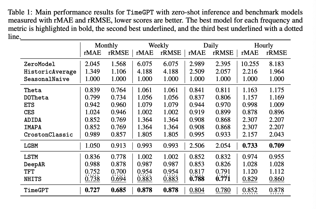
( No additional fine-tuning is performed on the test set )

TimeGPT

• Validity of a forecasting model can only be assessed relative to its performance against competing alternatives.
• Although accuracy is commonly seen as the only relevant metric, computational cost and implementation complexity are key factors for practical applications.

\(\rightarrow\) Results of TimeGPT are the result of a simple and extremely fast invocation of the prediction method of a pre-trained model.

( Other models require a complete pipeline for training and then predicting )

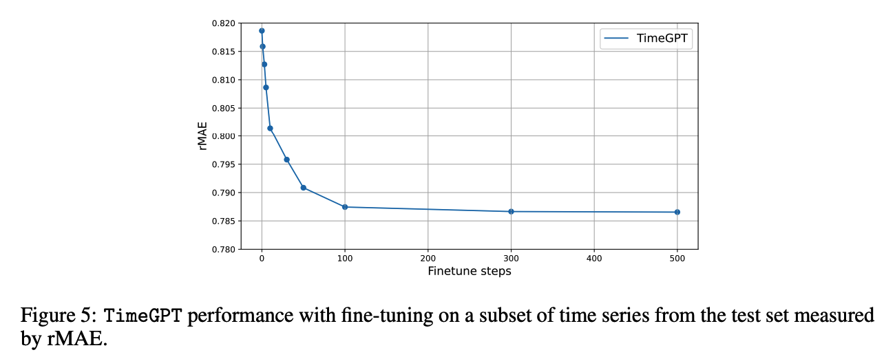
(2) Fine Tuning

(3) Time Comparison

Zero-shot inference

• average GPU inference speed of 0.6 milliseconds per series

  ( = nearly mirrors that of the simple Seasonal Naive )