Lag-Llama; Towards Foundation Models for Time Series Forecasting

Lag-Llama: Towards Foundation Models for Time Series Forecasting

Contents

1. Abstract
2. Introduction
3. Probabilistic TS Forecasting
4. Lag-Llama
5. Experiments

Abstract

Lag-Llama

• General-purpose univariate probabilistic TS forecasting model
• Trained on a large collection of TS data.
• Good zero-shot prediction capabilities on unseen “out-of-distribution” TS datasets
• Use smoothly broken power-laws to fit and predict model scaling behavior

( Code: https://github.com/kashif/pytorch-transformer-ts )

1. Introduction

Train a transformer model on a large collection of TS datasets and evaluate its performance on an unseen “out-of-distribution” dataset

( large collection of time series from the Monash Time Series Repository )

Experiments

• Test-set performance of this model on unseen time-series datasets
• Present a neural scaling laws study on the number of parameters and training data.

Contributions

1. Propose Lag-Llama

   • a model for univariate probabilistic time-series forecasting
   • suitable for scaling law analyses of TS foundation models

2. Train Lag-Llama on a corpus of TS datasets

   Test zero-shot on unseen time series datasets

   Identify a “stable” regime where the model constantly outperforms the baselines beyond a certain model size

3. Fit empirical scaling laws of the zero-shot test performance of the model as a function of the model size

   \(\rightarrow\) allowing us to potentially extrapolate and predict generalization beyond the models used in this paper.

2. Probabilistic TS Forecasting

Notation

• \(\mathcal{D}_{\text {train }}=\left\{x_{1: T^i}^i\right\}_{i=1}^D\),
  • at each time point \(t \in\left\{1, \ldots, T^i\right\}, x_t^i \in \mathbb{R}\)
• Goal: predict \(P \geq 1\) steps into the future
• \(\mathcal{D}_{\text {test }}=\left\{x_{T^i+1: T^i+P}\right\}_{i=1}^D\) or some held-out TS dataset
• Covariates \(\mathbf{c}_t^i\)
  • assumed to be non-stochastic and available in advance for the \(P\) future time points.

Univariate probabilistic time series forecasting

• \(p_{\mathcal{X}}\left(x_{t+1: t+P}^i \mid x_{1: t}^i, \mathbf{c}_{1: t+P}^i\right)\).

Sub-sample fixed context windows of size \(C \geq 1\)

• \(p_{\mathcal{X}}\left(x_{C+1: C+P}^i \mid x_{1: C}^i, \mathbf{c}_{1: C-1+P}^i\right)\).

Autoregressive model

• \(p_{\mathcal{X}}\left(x_{C+1: C+P}^i \mid x_{1: C}^i, \mathbf{c}_{1: C-1+P}^i ; \theta\right)=\prod_{t=C+1}^{C+P} p_{\mathcal{X}}\left(x_t^i \mid x_{1: t-1}^i, \mathbf{c}_{1: t-1}^i ; \theta\right)\).

3. Lag-Llama

(1) Lag Features

The only covariates we employ in this model are from the target values, in particular lag features

• lags are constructed from a set of appropriate lag indices for quarterly, monthly, weekly, daily, hourly, and second-level frequencies that correspond to the frequencies in our corpus of time series data

Lag

• Lag indices \(\mathcal{L}=\{1, \ldots, L\}\)

• Lag operation on a particular time value as \(x_t \mapsto \mathbf{c}_t \in \mathbb{R}^{ \mid \mathcal{L} \mid }\)

  • where each entry \(j\) of \(\mathbf{c}_t\) is given by \(\mathbf{c}_t[j]=x_{t-\mathcal{L}[j]}\).

• Thus to create lag features for some context-length window \(x_{1: C}\) …

  \(\rightarrow\) Need to sample a larger window with \(L\) more historical points denoted by \(x_{-L+1: C}\).

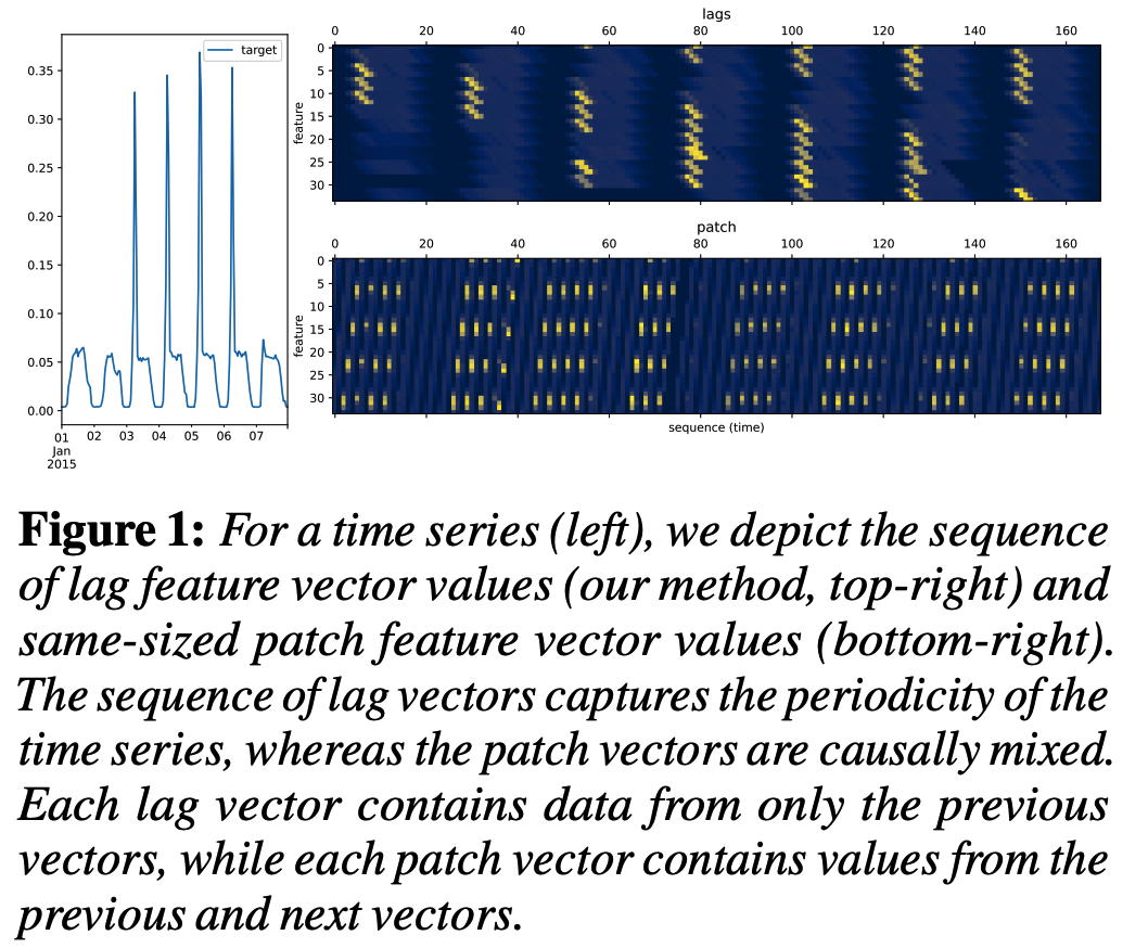
Other than lag, use overlapped patches

\(\rightarrow\) resulting in a sequence of vectors whose dimension can be specified

\(\rightarrow\) can lead to vectors whose entries are causally mixed. See Fig. 1 for an example of both approaches

Lag vs. Patch

• Both approaches essentially serve the same purpose

• Lag Pos

  • Indices of the lags correspond directly to the various possible seasonalities of the data

    \(\rightarrow\) advantage of preserving the date-time index causal structure

  • Can use masked decoders during training and autoregressive sampling at inference time

    ( which is not trivial with patches. )

• Lag Cons

  • Cownside to using lags is that it requires an \(L\)-sized or larger context window at inference time.

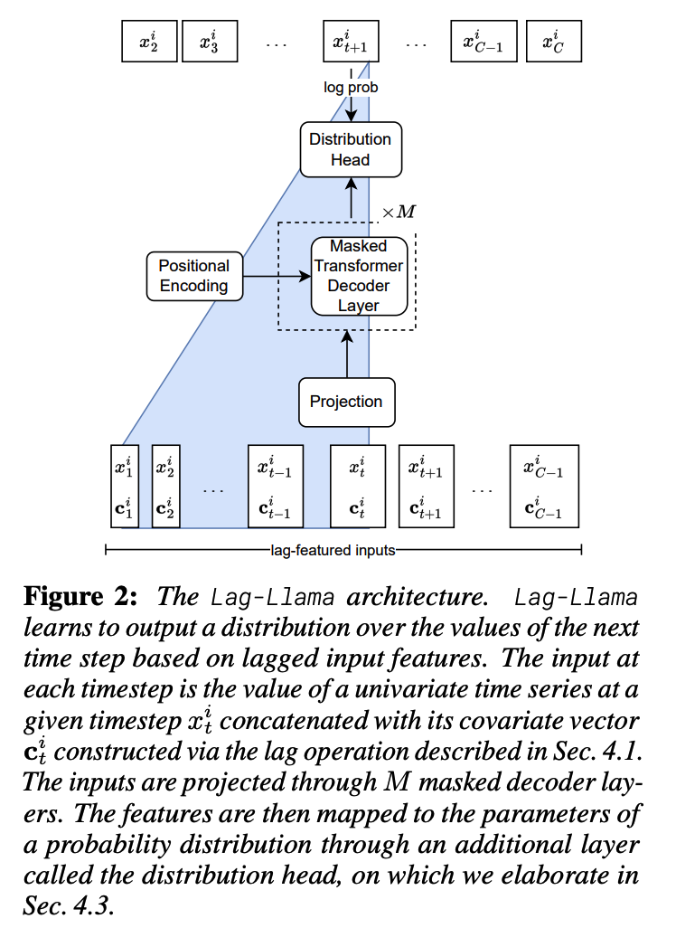
(2) Architecture

Based on the recent LlaMA [43] architecture

• incorporates prenormalization via the RMSNorm
• adds Rotary Positional Encoding (RoPE)
  • to each attention layer’s query and key representations.

Inference time

• Construct a feature vector

• Can obtain many samples from the predicted distribution

  & Concatenate them to the initial sequence to obtain further lag vectors

• ( via greedy autoregressive decoding ) Able to obtain many simulated trajectories

  \(\rightarrow\) Can calculate the uncertainty intervals for downstream decision-making tasks and metrics with respect to held-out data.

(3) Choice of Distribution Head

Last layer of Lag-Llama = Distribution head

• Projects the model’s features to the parameters of a probability distribution.
• Use Student’s \(t\)-distribution: output the three parameters corresponding to this distribution
  • degrees of freedom
  • mean
  • scale

(4) Value Scaling

Dataset can have any numerical magnitude11

\(\rightarrow\) Utilize the scaling heuristic from [36]

• For each univariate window, we calculate its
  • mean value \(\mu^i=\sum_{t=-L}^C x_t^i /(C+L)\)
  • variance \(\sigma^i\).
• Time series \(\left\{x_t^i\right\}_{t=-L}^C\) \(\rightarrow\) \(\left\{\left(x_t^i-\mu^i\right) / \sigma^i\right\}_{t=-L}^C\).
• Also incorporate \(\mu^i\) via \(\operatorname{sign}\left(\mu^i\right) \log \left(1+ \mid \mu^i \mid \right)\) as well as \(\log \left(\sigma^i\right)\) as time independent real-valued covariates.

During training and obtaining likelihood…

• the values are transformed using the mean and variance

During sampling…

• every timestep of data that is sampled is de-standardized using the same mean and variance.

(5) Augmentation

Freq-Mix & Freq-Mask

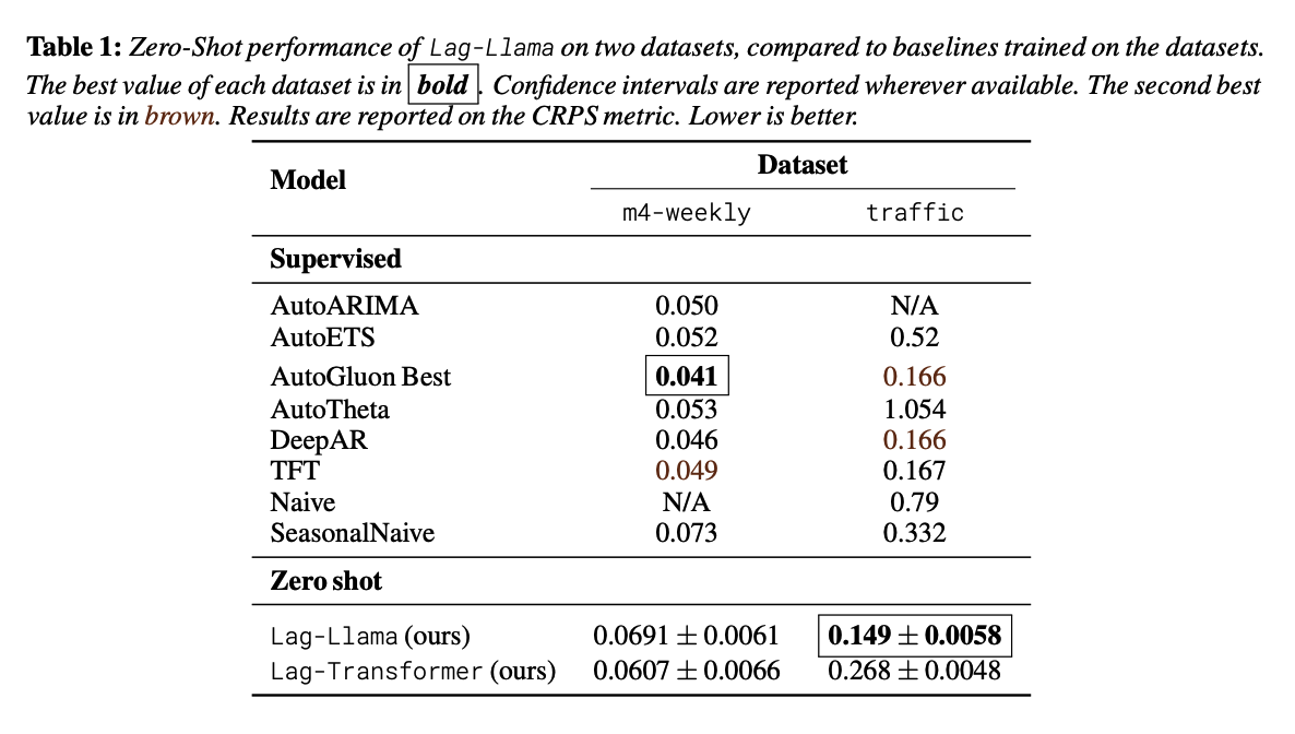
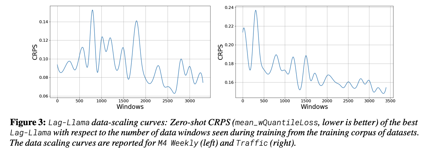
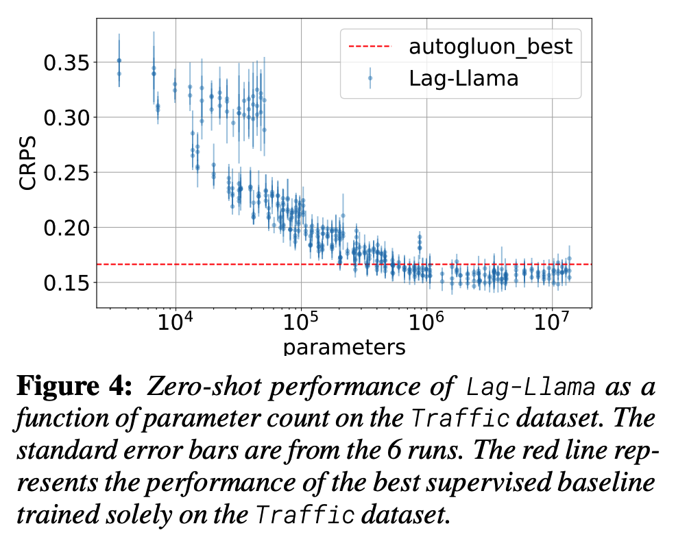
4. Experiments