Patch Diffusion; Faster and More Data-Efficient Training of Diffusion Models

Patch Diffusion: Faster and More Data-Efficient Training of Diffusion Models

Contents

1. Abstract
2. Patch Diffusion Training
   1. Patch-wise Score Matching
   2. Progressive and Stochastic Patch Size Scheduling
   3. Conditional Coordinates for Patch Location

Abstract

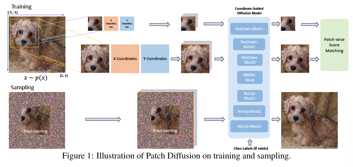
Patch Diffusion

• Generic patch-wise training framework
• Improve data efficiency
• Conditional score function at the patch level
• Two conditions
  • (1) Patch location is included as additional coordinate
  • (2) Patch size is randomized and diversified
    • to encode the cross-region dependency at multiple scales
• Achieve \(\gt\) 2x faster training

1. Patch Diffusion Training

Notation

• Dataset \(\left\{\boldsymbol{x}_n\right\}_{n=1}^N\), drawn from \(p(\boldsymbol{x})\).
• Perturbed distributions \(p_\sigma(\tilde{\boldsymbol{x}} \mid \boldsymbol{x})=\mathcal{N}(\tilde{\boldsymbol{x}} ; \boldsymbol{x}, \sigma \boldsymbol{I})\)
  • sequence of positive noise scales \(\sigma_{\min }=\sigma_0<\cdots<\sigma_t<\cdots<\sigma_T=\sigma_{\max }\),

Generalize to an infinite number of noise scale, \(T \rightarrow \infty\),

Forward diffusion process = SDE ( further converted to ODE )

• Closed form of the reverse SDE:
  • \(d \boldsymbol{x}=\left[\boldsymbol{f}(\boldsymbol{x}, t)-g^2(t) \nabla_{\boldsymbol{x}} \log p_{\sigma_t}(\boldsymbol{x})\right] d t+g(t) d \boldsymbol{w}\).
• Corresponding ODE of the reverse SDE ( = probability flow ODE )
  • \(d \boldsymbol{x}=\left[\boldsymbol{f}(\boldsymbol{x}, t)-0.5 g^2(t) \nabla_{\boldsymbol{x}} \log p_{\sigma_t}(\boldsymbol{x})\right] d t\).

Need to learn a function \(s_{\boldsymbol{\theta}}\left(\boldsymbol{x}, \sigma_t\right)\)

• ex) Denoising score matching
• After learning \(s_{\boldsymbol{\theta}}\left(\boldsymbol{x}, \sigma_t\right)\), we can obtain an estimated reverse SDE or ODE to collect data samples from the estimated data distribution.

Introduce our patch diffusion training in 3 subsections

• (1) Conditional score matching
  • On randomly cropped image patches
  • Condition: patch location & patch
• (2) Pixel coordinate systems
  • To provide better guidance on patch-level score matching
• (3) Sampling
  • w/o the need to explicitly sample separate local patches and merge them afterwards.

(1) Patch-wise Score Matching

Denoising score-matching

• Denoiser \(D_{\boldsymbol{\theta}}\left(\boldsymbol{x} ; \sigma_t\right)\)
  • Minimizes \(\mathbb{E}_{\boldsymbol{x} \sim p(\boldsymbol{x})} \mathbb{E}_{\boldsymbol{\epsilon} \sim \mathcal{N}\left(\mathbf{0}, \sigma_t^2 \boldsymbol{I}\right)} \mid \mid D_{\boldsymbol{\theta}}\left(\boldsymbol{x}+\boldsymbol{\epsilon} ; \sigma_t\right)-\boldsymbol{x} \mid \mid _2^2\).
• Score function : \(s_{\boldsymbol{\theta}}\left(\boldsymbol{x}, \sigma_t\right)=\left(D_{\boldsymbol{\theta}}\left(\boldsymbol{x} ; \sigma_t\right)-\boldsymbol{x}\right) / \sigma_t^2\)

Denoising score-matching + Patchify

• Step 1) Randomly crop small patches \(\boldsymbol{x}_{i, j, s}\),
  • \((i, j)\) : location of patch & \(s\) : patch size
• Step 2) Minimize
  • \(\mathbb{E}_{\boldsymbol{x} \sim p(\boldsymbol{x}), \boldsymbol{\epsilon} \sim \mathcal{N}\left(\mathbf{0}, \sigma_t^2 \boldsymbol{I}\right),(i, j, s) \sim \mathcal{U}} \mid \mid D_{\boldsymbol{\theta}}\left(\tilde{\boldsymbol{x}}_{i, j, s} ; \sigma_t, i, j, s\right)-\boldsymbol{x}_{i, j, s} \mid \mid _2^2\).
    • where \(\tilde{\boldsymbol{x}}_{i, j, s}=\boldsymbol{x}_{i, j, s}+\boldsymbol{\epsilon}\) and \(\mathcal{U}\) denotes the uniform distn

• Conditional score function : \(s_{\boldsymbol{\theta}}\left(\boldsymbol{x}, \sigma_t, i, j, s\right)\), is defined on each local patch

  \(\rightarrow\) Learn the scores for pixels within each image patch

  • conditioning on its location and patch size

Challenge : score function \(s_{\boldsymbol{\theta}}\left(\boldsymbol{x}, \sigma_t, i, j, s\right)\) has only seen local patches

( may have not captured the global cross-region dependency between local patches )

Solution:

• (1) Random patch sizes
  • sampled from a mixture of small and large patch sizes
  • cropped large patch could be seen as a sequence of small patches
• (2) Involving a small ratio of full-size images
  • in some iterations during training, full-size images are required to be seen.

(2) Progressive and Stochastic Patch Size Scheduling

Propose patch-size scheduling

\(s \sim p_s:= \begin{cases}p & \text { when } s=R, \\ \frac{3}{5}(1-p) & \text { when } s=R / / 2, \\ \frac{2}{5}(1-p) & \text { when } s=R / / 4 .\end{cases}\).

Two patch-size schedulings

• (1) Stochastic:
  • randomly sample \(s \sim p_s\) for each mini-batch
• (2) Progressive
  • from small patches to large patches

(3) Conditional Coordinates for Patch Location

( Motivated by COCO-GAN )

Incorporate and simplify the conditions of patch locations in the score function

\(\rightarrow\) Pixel-level coordinate system

• normalize the pixel coordinate values to \([-1,1]\)

• concatenate the two coordinate channels with the original image channels

( = input of our denoiser \(D_{\boldsymbol{\theta}}\). )

When computing the loss … ignore the reconstructed coordinate channels

( = only minimize the loss on the image channels )