Understanding Diffusion Objectives as the ELBO with Simple Data Augmentation

Understanding Diffusion Objectivevs as the ELBO with Simple Ddata Augmentation

Contents

1. Abstract
2. Introduction
3. Model
   1. Forward process and noise schedule
   2. Generative Model
4. Diffusion Model Objectives
   1. The weighted loss
   2. Invariance of the weighted loss to the noise schedule \(\lambda_t\)
5. Weighted Loss as the ELBO with DA

0. Abstract

SOTA Diffusion models

• optimized with objectives that typically look very different from the MLE and ELBO

This paper: reveal that diffusion model objectives are actually closely related to the ELBO

Diffusion model objectives

= weighted integral of ELBOs over different noise levels

• weight: depends on the specific objective used

Monotonic weighting: Diffusion objective = ELBO

• combined with simple data augmentation, namely Gaussian noise perturbation

1. Introduction

Application of diffusion model

• text-to-image generation
• image-to-image generation
• text-to-speech
• density estimation

Diffusion models

= Special case of deep VAE

• with a particular choice of inference model and generative model.

Optimization of diffusion models

• by maximizing the ELBO ( just like VAE)
• ELBO for short. It was shown by Variational Diffusion Models (VDM) [Kingma et al., 2021] and [Song et al., 2021a] how to optimize continuous-time diffusion models with the ELBO objective

HOWEVER … best results were achieved with other objectives

• ex) Denoising score matching objective [Song and Ermon, 2019]
• ex) Simple noise-prediction objective [Ho et al., 2020]

\(\rightarrow\) Looks very different from the traditionally popular maximum likelihood and ELBO

\(\rightarrow\) This paper reveals that all training objective used in SOTA diffusion models are actually closely related to the ELBO objective

Section outline

• [Section 2] Broad diffusion model family

• [Section 3] Various diffusion model objectives

  = Special cases of a weighted loss with different choices of weighting

  • Weighting function specifies the weight per noise level
  • [Section 3.2] During training, the noise schedule acts as a importance sampling distribution for estimating the loss, and is thus important for efficient optimization.

  \(\rightarrow\) Based on this insight we propose a simple adaptive noise schedule

• [Section 4] Main result

  • If the weighting function is a monotonic function of time…

    Weighted loss = Maximizing the ELBO with data augmentation ( Gaussian noise perturbation ) .

• [Section 5] Experiments with various new monotonic weights on the ImageNet dataset

(1) Related Work

Variational Diffusion Models

• showed how to optimize continous-time diffusion models towards the ELBO

(This paper) Generalize these earlier results by showing that any diffusion objective that corresponds with monotonic weighting corresponds to the ELBO, combined with a form of DistAug

• DistAug : method of training data distribution augmentation for generative models, where model is
  • conditioned on the data augmentation parameter at training time
  • conditioned on ’no augmentation’ at inference time
• Additive Gaussian noise
  • form of data distribution smoothing

2. Model

Notation

• Dataset distribution: \(q(\mathbf{x})\).
• Generative mode: \(p_{\boldsymbol{\theta}}(\mathbf{x})\)
  • shorthand notation \(p:=p_{\boldsymbol{\theta}}\).
• Observed variable: \(\mathbf{x}\)
  • output of a pre-trained encoder, as in latent diffusion models
• Latent variables: \(\mathbf{z}_t\) for timesteps \(t \in[0,1]\) : \(\mathbf{z}_{0, \ldots, 1}:=\mathbf{z}_0, \ldots, \mathbf{z}_1\).

Forward & Backward

• [Forward] Forward process forming a conditional joint distribution \(q\left(\mathbf{z}_{0, \ldots, 1} \mid \mathbf{x}\right)\)
• [Backward] Generative model forming a joint distribution \(p\left(\mathbf{z}_{0, \ldots, 1}\right)\).

(1) Forward process and noise schedule

Forward process = Gaussian diffusion process

• Conditional distribution \(q\left(\mathbf{z}_{0, \ldots, 1} \mid \mathbf{x}\right)\)
• Marginal distribution \(q\left(\mathbf{z}_t \mid \mathbf{x}\right)\)
  • \(\mathbf{z}_t=\alpha_\lambda \mathbf{x}+\sigma_\lambda \boldsymbol{\epsilon} \text { where } \boldsymbol{\epsilon} \sim \mathcal{N}(0, \mathbf{I})\).

Variance preserving (VP) forward process

• \(\alpha_\lambda^2=\operatorname{sigmoid}\left(\lambda_t\right)\) ,
• \(\sigma_\lambda^2=\) sigmoid \(\left(-\lambda_t\right)\),

( other choices are possible )

Log signal-to-noise ratio ( \(\log\)-SNR)

• \(\lambda=\log \left(\alpha_\lambda^2 / \sigma_\lambda^2\right)\).

Noise schedule

• Strictly monotonically decreasing function \(f_\lambda\)

• Maps from the time variable \(t \in[0,1]\) to the corresponding log-SNR \(\lambda: \lambda=f_\lambda(t)\).
• Denote the log-SNR as \(\lambda_t\) to emphasize that it is a function of \(t\).
• Endpoints of the noise schedule
  • \(\lambda_{\max }:=f_\lambda(0)\) .
  • \(\lambda_{\min }:=f_\lambda(1)\).

Due to its monotonicity, \(f_\lambda\) is invertible: \(t=f_\lambda^{-1}(\lambda)\).

• can do change of variables

a) Model training

• Sample time \(t\) uniformly: \(t \sim \mathcal{U}(0,1)\),
• Compute \(\lambda=f_\lambda(t)\).
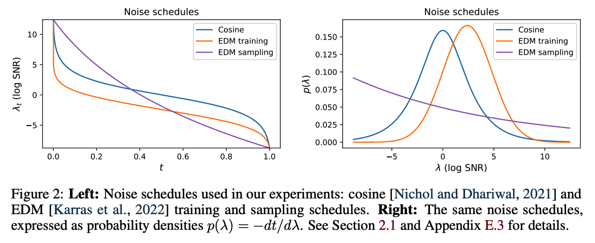
• Results: Distribution over noise levels \(p(\lambda)=-d t / d \lambda=-1 / f_\lambda^{\prime}(t)\)

b) Sampling

• Sometimes it is best to use a different noise schedule for sampling from the model than for training.

• Density \(p(\lambda)\) gives the relative amount of time the sampler spends at different noise levels.

(2) Generative Model

Notation

• Data \(\mathbf{x} \sim \mathcal{D}\), with density \(q(\mathbf{x})\),
• Forward model : defines a joint distribution \(q\left(\mathbf{z}_0, \ldots, \mathbf{z}_1\right)=\) \(\int q\left(\mathbf{z}_0, \ldots, \mathbf{z}_1 \mid \mathbf{x}\right) q(\mathbf{x}) d \mathbf{x}\),
  • Marginals \(q_t(\mathbf{z}):=q\left(\mathbf{z}_t\right)\).
• Generative model
  • defines a corresponding joint distribution over latent variables: \(p\left(\mathbf{z}_0, \ldots, \mathbf{z}_1\right)\).

log-SNR \(\lambda: \lambda=f_\lambda(t)\).

• For large enough \(\lambda_{\max }\)
  • \(\mathbf{z}_0\) is almost identical to \(\mathbf{x}\),
  • Learning a model \(p\left(\mathbf{z}_0\right)\) \(\approx\) Learning a model \(p(\mathbf{x})\).
• For small enough \(\lambda_{\min }\)
  • \(\mathbf{z}_1\) holds almost no information about \(\mathbf{x}\),
  • There exists a distribution \(p\left(\mathbf{z}_1\right)\) satisfying \(D_{K L}\left(q\left(\mathbf{z}_1 \mid \mathbf{x}\right) \mid \mid p\left(\mathbf{z}_1\right)\right) \approx 0\).
    • Usually we can use \(p\left(\mathbf{z}_1\right)=\mathcal{N}(0, \mathbf{I})\).

Score model: \(\mathbf{s}_{\boldsymbol{\theta}}(\mathbf{z} ; \lambda)\)

• Approximate \(\nabla_{\mathbf{z}} \log q_t(\mathbf{z})\)
• If \(\mathbf{s}_{\boldsymbol{\theta}}(\mathbf{z} ; \lambda)=\nabla_{\mathbf{z}} \log q_t(\mathbf{z})\), then the forward process can be exactly reversed

If \(D_{K L}\left(q\left(\mathbf{z}_1\right) \mid \mid p\left(\mathbf{z}_1\right)\right) \approx 0\) and \(\mathbf{s}_{\boldsymbol{\theta}}(\mathbf{z} ; \lambda) \approx \nabla_{\mathbf{z}} \log q_t(\mathbf{z})\), then we have a good generative model

\(\rightarrow\) So, our generative modeling task is reduced to learning a score network \(\mathbf{s}_{\boldsymbol{\theta}}(\mathbf{z} ; \lambda)\) that approximates \(\nabla_{\mathbf{z}} \log q_t(\mathbf{z})\).

Sampling from the generative model

• By sampling \(\mathbf{z}_1 \sim p\left(\mathbf{z}_1\right)\), then solving the reverse SDE using the estimated \(\mathbf{s}_{\boldsymbol{\theta}}(\mathbf{z} ; \lambda)\).

• ( Recent diffusion models ) Sophisticated procedures for approximating the reverse SDE

3. Diffusion Model Objectives

a) Denoising score matching

Learn a score network \(\mathbf{s}_{\boldsymbol{\theta}}\left(\mathbf{z} ; \lambda_t\right)\) for all noise levels \(\lambda_t\).

\(\rightarrow\) Can beachieved by minimizing a denoising score matching objective

• over all noise scales
• and all datapoints \(\mathbf{x} \sim \mathcal{D}\)

Denoising score matching objective

\(\mathcal{L}_{\mathrm{DSM}}(\mathbf{x})=\mathbb{E}_{t \sim \mathcal{U}(0,1), \boldsymbol{\epsilon} \sim \mathcal{N}(0, \mathbf{I})}\left[\tilde{w}(t) \cdot \mid \mid \mathbf{s}_{\boldsymbol{\theta}}\left(\mathbf{z}_t, \lambda_t\right)-\nabla_{\mathbf{z}_t} \log q\left(\mathbf{z}_t \mid \mathbf{x}\right) \mid \mid _2^2\right]\),

• where \(\mathbf{z}_t=\alpha_\lambda \mathbf{x}+\sigma_\lambda \boldsymbol{\epsilon}\).

b) \(\epsilon\)-prediction objective

Score network : typically parameterized through a noise-prediction ( \(\boldsymbol{\epsilon}\)-prediction) model:

• \(\mathbf{s}_{\boldsymbol{\theta}}(\mathbf{z} ; \lambda)=-\hat{\boldsymbol{\epsilon}}_{\boldsymbol{\theta}}(\mathbf{z} ; \lambda) / \sigma_\lambda\).

Noise-prediction loss

\(\mathcal{L}_{\boldsymbol{\epsilon}}(\mathbf{x})=\frac{1}{2} \mathbb{E}_{t \sim \mathcal{U}(0,1), \boldsymbol{\epsilon} \sim \mathcal{N}(0, \mathbf{I})}\left[ \mid \mid \hat{\epsilon}_\theta\left(\mathbf{z}_t ; \lambda_t\right)-\epsilon \mid \mid _2^2\right]\).

Since \(\mid \mid \mathbf{s}_{\boldsymbol{\theta}}\left(\mathbf{z}_t, \lambda_t\right)-\nabla_{\mathbf{x}_t} \log q\left(\mathbf{z}_t \mid \mathbf{x}\right) \mid \mid _2^2=\sigma_\lambda^{-2} \mid \mid \hat{\boldsymbol{\epsilon}}_{\boldsymbol{\theta}}\left(\mathbf{z}_t ; \lambda_t\right)-\boldsymbol{\epsilon} \mid \mid _2^2\) …

\(\rightarrow\) Noise-prediction loss is simply a version of the denoising score matching objective

• where \(\tilde{w}(t)=\sigma_t^2\).

Ho et al. [2020]

• showed that this noise-prediction objective can result in high-quality samples

Dhariwal and Nichol [2022]

• switch from a ‘linear’ to a ‘cosine’ noise schedule \(\lambda_t\)

c) ELBO

[Kingma et al., 2021, Song et al., 2021a]

ELBO of continuous-time diffusion models simplifies to ..

\(-\operatorname{ELBO}(\mathbf{x})=\frac{1}{2} \mathbb{E}_{t \sim \mathcal{U}(0,1), \boldsymbol{\epsilon} \sim \mathcal{N}(0, \mathbf{I})}\left[-\frac{d \lambda}{d t} \cdot \mid \mid \hat{\epsilon}_\theta\left(\mathbf{z}_t ; \lambda_t\right)-\epsilon \mid \mid _2^2\right]+c\).

(1) The weighted loss

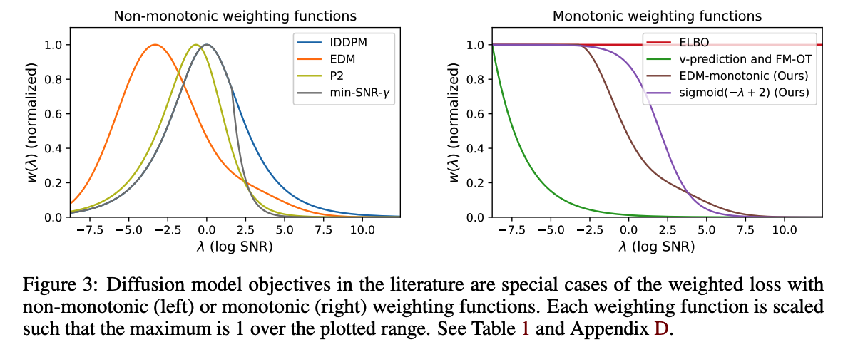
Objective functions used in practice

= special cases of a weighted loss introduced by Kingma with a particular choice of weighting function \(w\left(\lambda_t\right):\)

\(\mathcal{L}_w(\mathbf{x})=\frac{1}{2} \mathbb{E}_{t \sim \mathcal{U}(0,1), \boldsymbol{\epsilon} \sim \mathcal{N}(0, \mathbf{I})}\left[w\left(\lambda_t\right) \cdot-\frac{d \lambda}{d t} \cdot \mid \mid \hat{\epsilon}_\theta\left(\mathbf{z}_t ; \lambda_t\right)-\epsilon \mid \mid _2^2\right]\)

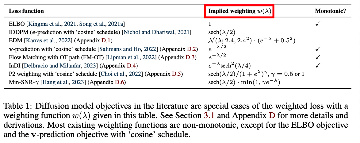
Examples)

• ex) ELBO = uniform weighting, i.e. \(w\left(\lambda_t\right)=1\).
• ex) Noise-prediction objective = \(w\left(\lambda_t\right)=-1 /(d \lambda / d t)\).
  • More compactly expressed as \(w\left(\lambda_t\right)=p\left(\lambda_t\right)\),
    • i.e., the PDF of the implied distribution over noise levels \(\lambda\) during training.
  • Often used with the cosine schedule \(\lambda_t\),
    • which implies \(w\left(\lambda_t\right) \propto \operatorname{sech}\left(\lambda_t / 2\right)\).

(2) Invariance of the weighted loss to the noise schedule \(\lambda_t\)

Kingma et al. [2021]

• ELBO is invariant to the choice of noise schedule

  ( except for its endpoints \(\lambda_{\min }\) and \(\lambda_{\max }\). )

General weighted diffusion loss

• with a change of variables from \(t\) to \(\lambda\)

\(\mathcal{L}_w(\mathbf{x})=\frac{1}{2} \int_{\lambda_{\min }}^{\lambda_{\max }} w(\lambda) \mathbb{E}_{\boldsymbol{\epsilon} \sim \mathcal{N}(0, \mathbf{I})}\left[ \mid \mid \hat{\boldsymbol{\epsilon}}_{\boldsymbol{\theta}}\left(\mathbf{z}_\lambda ; \lambda\right)-\boldsymbol{\epsilon} \mid \mid _2^2\right] d \lambda\)

Meaning

• Shape of the function \(f_\lambda\) between \(\lambda_{\min }\) and \(\lambda_{\max }\) does not affect the loss

• Only the weighting function \(w(\lambda)\) affects!

Monte Carlo estimator

• This invariance does not hold for the Monte Carlo estimator of the loss, based on random samples \(t \sim \mathcal{U}(0,1), \boldsymbol{\epsilon} \sim \mathcal{N}(0, \mathbf{I})\).

• Noise schedule still affects the variance of this Monte Carlo estimator and its gradients;

  \(\rightarrow\) Affects the efficiency of optimization

• Noise schedule acts as an importance sampling distribution for estimating the loss integral

Rewrite the weighted loss

• Note that \(p(\lambda)=-1 /(d \lambda / d t)\).
• Clarifies the role of \(p(\lambda)\) as an importance sampling distribution:

\(\mathcal{L}_w(\mathbf{x})=\frac{1}{2} \mathbb{E}_{\boldsymbol{\epsilon} \sim \mathcal{N}(0, \mathbf{I}), \lambda \sim p(\lambda)}\left[\frac{w(\lambda)}{p(\lambda)} \mid \mid \hat{\boldsymbol{\epsilon}}_{\boldsymbol{\theta}}\left(\mathbf{z}_\lambda ; \lambda\right)-\epsilon \mid \mid _2^2\right]\)

4. Weighted Loss as the ELBO with DA