Self-supervised Contrastive Forecasting

Self-supervised Contrastive Forecasting

https://openreview.net/pdf?id=nBCuRzjqK7

Contents

1. Abstract
2. Introduction
3. Related Work
4. Method
5. Experiments

Abstract

Challenges of Long-term forecasting

• Time and memory complexity of handling long sequences

• Existing methods

  • Rely on sliding windows to process long sequences

    \(\rightarrow\) Struggle to effectively capture long-term variations

    ( \(\because\) Partially caught within the short window )

Self-supervised Contrastive Forecasting

• Overcomes this limitation by employing…

  • (1) contrastive learning
  • (2) enhanced decomposition architecture

  ( specifically designed to focus on long-term variations )

[1] Proposed contrastive loss

• Incorporates global autocorrelation held in the whole TS
  • facilitates the construction of positive and negative pairs in a self-supervised manner.

[2] Decomposition networks

https://github.com/junwoopark92/Self-Supervised-Contrastive-Forecsating.

1. Introduction

Sliding window approach

• enables models to not only process the long-time series
• but also capture local dependencies between the past and future sequence within the windows,

\(\rightarrow\) Accurate short-term predictions

a) Transformer & CNN

• [1] Transformer-based models
  • Reduced computational costs of using long windows
• [2] CNN-based models
  • Applied a dilation in convolution operations to learn more distant dependencies while benefiting from their efficient computational cost.

\(\rightarrow\) Effectiveness in long-term forecasting remains uncertain

b) Findings

Analyze the limitations of existing models trained with sub-sequences (i.e., based on sliding windows) for long-term forecasting tasks.

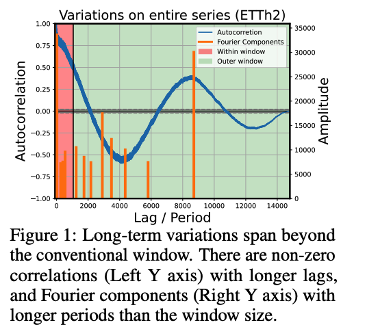
• Observed that most TS often contain long-term variations with periods longer than conventional window lengths …. [Figure 1, 5]

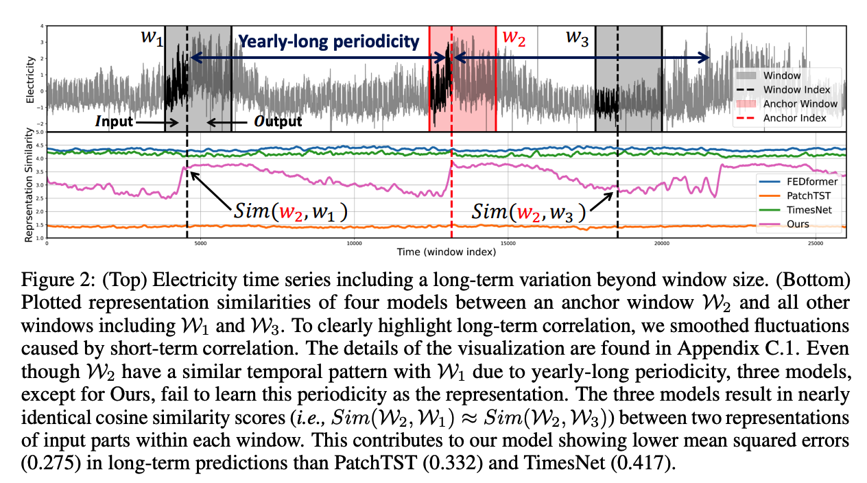
• If a model successfully captures these long-term variations. ….

  \(\rightarrow\) Representations of two distant yet correlated windows to be more similar than uncorrelated ones

c) Limitation of previous works

• Treat each window independently during training

  \(\rightarrow\) Challenging for the model to capture such long-term variations across distinct windows

• [Figure 2]

  • Fail to reflect the long-term correlations between two distant windows
  • Overlook long-term variations by focusing more on learning short-term variations within the window

d) Previous works

[1] Decomposition approaches (Zeng et al., 2023; Wang et al., 2023)

• Often treat the long-term variations partially caught in the window as simple non-periodic trends and employ a linear model to extend the past trend into the prediction.

[2] Window-unit normalization methods (Kim et al., 2021; Zeng et al., 2023)

• Hinder long-term prediction by normalizing numerically significant values (e.g., maximum, minimum, domain-specific values in the past) that may have a long-term impact on the TS

• But still …. normalization methods are essential for mitigating distribution shift

  \(\rightarrow\) *New approach is necessary to learn long-term variations while still keeping the normalization methods

e) Proposal: AutoCon

Novel contrastive learning to help the model capture long-term dependencies that exist across different windows.

Idea: Mini-batch can consist of windows that are temporally far apart

• Interval between windows to span the entire TS length

  ( = much longer than the window length )

f) Section Outline

Contrastive loss

• Combination with a decomposition-based model architecture
  • consists two branches: (1) short-term branch & (2) long-term branch
• CL loss is applied to the long-term branch
  • Previous work: long-term branch = single linear layer
    • Unsuitable for learning long-term representations
  • Redesign the decomposition architecture where the long-term branch has sufficient capacity to learn long-term representation from our loss.

g) Main contributions

• Long-term performances of existing models are poor
  • \(\because\) Overlooked the long-term variations beyond the window
• Propose AutoCon
  • Novel contrastive loss function to learn a long-term representation by constructing positive and negative pairs across distant windows in a self-supervised manner
• Extensive experiments

2. Related work

(1) CL for TSF

Numerous methods (Tonekaboni et al., 2021; Yue et al., 2022; Woo et al., 2022a)

How to construct positive pairs ?

• Temporal consistency (Tonekaboni et al., 2021)
• Subseries consistency (Franceschi et al., 2019)
• Contextual consistency (Yue et al., 2022).

\(\rightarrow\) Limitation in that only temporally close samples are selected as positives

=> Overlooking the periodicity in the TS

CoST (Woo et al., 2022a): consider periodicity through Frequency Domain Contrastive loss

• Still …. could not consider periodicity beyond the window length

  ( \(\because\) Still uses augmentation for the window )

This paper: Randomly sampled sequences in a batch can be far from each other in time

\(\rightarrow\) Propose a novel selection strategy to choose

• not only (1) local positive pairs
• but also (2) global positive pairs

(2) Decomposition for LTSF

Numerous methods (Wu et al., 2021; Zhou et al., 2022b; Wang et al., 2023)

• offer robust and interpretable predictions

DLinear (Zeng et al., 2023)

• Exceptional performance by using a decomposition block and a single linear layer for each trend and seasonal component.

• Limitation

  • Only effective in capturing high-frequency components that impact short-term predictions
  • Miss low-frequency components that significantly affect long-term predictions

  \(\rightarrow\) A single linear model may be sufficient for short-term prediction! ( =Inadequate for long-term prediction )

3. Method

Notation

Forecasting task: Sliding window approach

• Covers all possible in-output sequence pairs of the entire TS \(\mathcal{S}=\left\{\mathbf{s}_1, \ldots, \mathbf{s}_T\right\}\)

  • \(T\) : Length of the observed TS

  • \(\mathbf{s}_t \in \mathbb{R}^c\) : Observation with \(c\) dimension.

    ( set the dimension \(c\) to 1 )

• Sliding a window with a fixed length \(W\) on \(\mathcal{S}\),

  \(\rightarrow\) Obtain the windows \(\mathcal{D}=\left\{\mathcal{W}_t\right\}_{t=1}^M\) where \(\mathcal{W}_t=\left(\mathcal{X}_t, \mathcal{Y}_t\right)\) are divided into two parts:

  • \(\mathcal{X}_t=\) \(\left\{\mathbf{s}_t, \ldots, \mathbf{s}_{t+I-1}\right\}\) .
  • \(\mathcal{Y}_t=\left\{\mathbf{s}_{t+I}, \ldots, \mathbf{s}_{t+I+O-1}\right\}\) .

• Global index sequence of \(\mathcal{W}_t\) as \(\mathcal{T}_t=\{t+i\}_{i=0}^{W-1}\).

(1) Autocorrelation-based Contrastive Loss for LTSF

a) Missing Long-term Dependency in the Window

Forecasting model : struggle to predict long-term variations

\(\because\) They are not captured within the window.

Step 1) Identify these long-term variations using autocorrelation

( Inspired by the stochastic process theory )

( Notation: Real discrete-time process \(\left\{\mathcal{S}_t\right\}\) )

• Autocorrelation function

  \(\mathcal{R}_{\mathcal{S}}(h)\): \(\mathcal{R}_{\mathcal{S S}}(h)=\lim _{T \rightarrow \infty} \frac{1}{T} \sum_{t=1}^T \mathcal{S}_t \mathcal{S}_{t-h}\)

  • Correlation between observations at different times (i.e., time lag \(h\) ).
  • Range [-1,1] … indicates that all points separated by \(h\) in the series \(\mathcal{S}\) are linearly related ( positive or negative )

• Previous works

  • Have also leveraged autocorrelation

  • However, only apply it to capture variations within the window

    ( overlooking long-term variations that span beyond the window )

\(\rightarrow\) Propose a representation learning method via CL to capture these long-term variations quantified by the “GLOBAL” autocorrelation

Step 2) Autocorrelation-based Contrastive Loss (AutoCon)

• Mini-batch can consist of windows that are temporally very far apart
• Time distance can be as long as the entire series length \(T\) ( » window length \(W\) )
• Address long-term dependencies that exist throughout the entire TS by establishing relationships between windows

Relationship between the two windows

• Based on the global autocorrelation
• Two windows \(\mathcal{W}_{t_1}\) and \(\mathcal{W}_{t_2}\)
  • each have \(W\) observations with globally indexed time sequence \(\mathcal{T}_{t_1}=\left\{t_1+i\right\}_{i=0}^{W-1}\) and \(\mathcal{T}_{t_2}=\left\{t_2+j\right\}_{j=0}^{W-1}\).
• Time distances between all pairs of two observations: matrix \(\boldsymbol{D} \in \mathbb{R}^{W \times W}\).
  • Contains time distance as elements \(\boldsymbol{D}_{i, j}= \mid \left(t_2+j\right)-\left(t_1+i\right) \mid\).
  • Global autocorrelation: \(r\left(\mathcal{T}_{t_1}, \mathcal{T}_{t_2}\right)= \mid \mathcal{R}_{\mathcal{S S}}\left( \mid t_1-t_2 \mid \right) \mid\).
    • \(\mathcal{R}_{\mathcal{SS}}\) : global autocorrelation calculated from train series \(\mathcal{S}\).

Similarities between all pairs of window representations

• follow the global autocorrelation measured in the data space

• Define positive and negative samples in a relative manner inspired by SupCR (Zha et al., 2022)

• SupCR (Zha et al., 2022) vs. AutoCon

  • SupCR: uses annotated labels to determine the relationship between images

  • AutoCon: use the global autocorrelation \(\mathcal{R}_{\mathcal{S}}\) to determine the relationship between windows

    \(\rightarrow\) making our approach an unsupervised method

Notation

• Mini-batch \(\mathcal{X} \in \mathbb{R}^{N \times I}\) consisting of \(N\) windows
• Representations \(\boldsymbol{v} \in \mathbb{R}^{N \times I \times d}\) where \(\boldsymbol{v}=\operatorname{Enc}(\mathcal{X}, \mathcal{T})\).
• AutoCon: computed over the representations \(\left\{\boldsymbol{v}^{(i)}\right\}_{i=1}^N\) with the corresponding time sequence \(\left\{\mathcal{T}^{(i)}\right\}_{i=1}^N\) as:

\(\mathcal{L}_{\text {AutoCon }}=-\frac{1}{N} \sum_{i=1}^N \frac{1}{N-1} \sum_{j=1, j \neq i}^N r^{(i, j)} \log \frac{\exp \left(\operatorname{Sim}\left(\boldsymbol{v}^{(i)}, \boldsymbol{v}^{(j)}\right) / \tau\right)}{\sum_{k=1}^N \mathbb{1}_{\left[k \neq i, r^{(i, k)} \leq r^{(i, j)}\right]} \exp \left(\operatorname{Sim}\left(\boldsymbol{v}^{(i)}, \boldsymbol{v}^{(k)}\right) / \tau\right)}\).

(2) Decomposition Architecture for Long-term Representation

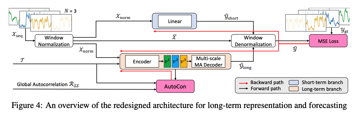
Existing models : commonly adopt the decomposition architecture

• seasonal branch and a trend branch

This paper

• Trend branch = long-term branch
• Seasonal branch = short-term branch

AutoCon

• Designed to learn long-term representations
  • Not to use it in the short-term branch to enforce long-term dependencies
• Integrating (1) AutoCon + (2) current decomposition architecture: Challenging
  • Reason 1) Both branches share the same representation
  • Reason 2) Long-term branch consists of a linear layer
    • not suitable for learning representations
  • Recent linear-based models (Zeng et al., 2023) outperform complicated DL models at short-term predictions
    • doubts whether a DL model is necessary to learn the high-frequency variations.

Redesign a model architecture

• Both temporal locality for short-term and globality for long-term forecasting

• Decomposition Architecture: 3 main features

  • (1) Normalization and Denormalization for Nonstationarity

    • Window-unit normalization & denormalization
    • \(\mathcal{X}_{\text {norm }}=\mathcal{X}-\overline{\mathcal{X}}, \quad \mathcal{Y}_{\text {pred }}=\left(\mathcal{Y}_{\text {short }}+\mathcal{Y}_{\text {long }}\right)+\overline{\mathcal{X}}\).

  • (2) Short-term Branch for Temporal Locality

    • Short-period variations :
      • often repeat multiple times within the input sequence
      • exhibit similar patterns with temporally close sequences
    • This locality of short-term variations supports the recent success of linear-based models
    • \(\mathcal{Y}_{\text {short }}=\operatorname{Linear}\left(\mathcal{X}_{\text {norm }}\right)\).

  • (3) Long-term Branch for Temporal Globality

    • Designed to apply the AutoCon method

    • Employs an encoder-decoder architecture

      • [Encoder] with sufficient capacity: \(\boldsymbol{v}=\operatorname{Enc}\left(\mathcal{X}_{\text {norm }}, \mathcal{T}\right)\).

        • to learn the long-term presentation leverages both sequential information and global information (i.e., timestampbased features derived from \(\mathcal{T}\) )
        • use TCN for its computational efficiency

      • [Decoder] multi-scale Moving Average (MA) block (Wang et al., 2023)

        • with different kernel sizes \(\left\{k_i\right\}_{i=1}^n\)
          • to capture multiple periods
        • \(\hat{\mathcal{Y}}_{\text {long }}=\frac{1}{n} \sum_{i=1}^n \operatorname{AvgPool}(\operatorname{Padding}(M L P(\boldsymbol{v})))_{k_i}\).
        • The MA block at the head of the long-term branch smooths out short-term fluctuations, naturally encouraging the branch to focus on long-term information

Objective function \(\mathcal{L}\) :

• \(\mathcal{L}=\mathcal{L}_{\text {MSE }}+\lambda \cdot \mathcal{L}_{\text {AutoCon }}\).

4. Experiments

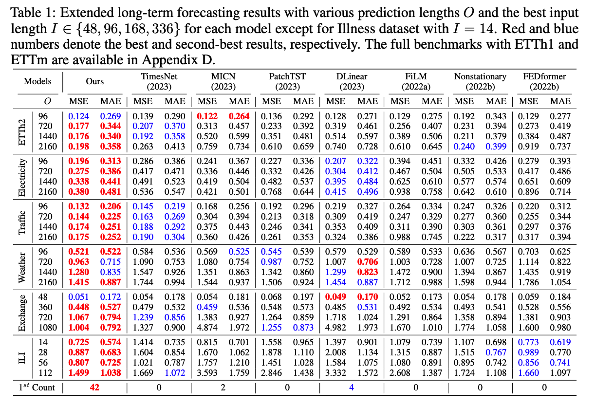
(1) Main Results

a) Extended Long-term Forecasting

b) Dataset Analysis

Goal : Learn long-term variations

Performance improvements of our model = affected by the magnitude and the number of long-term variations

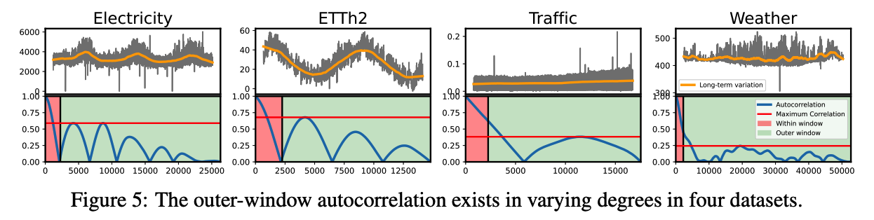
[Figure 5]

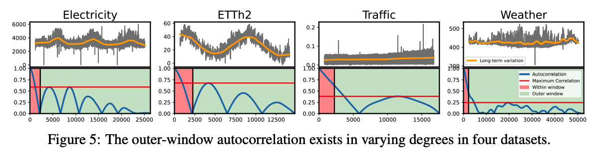
• Various yearly-long business cycles and natural cycles
• ex) ETTh2 and Electricity
  • Strong long-term correlations with peaks at several lags repeated multiple times.
  • Thus, AutoCOnexhibited significant performance gain s, which are 34% and 11% reduced error compared to the second-best model
• ex) Weather
  • Relatively lower correlations outside the windows
  • Least improvement with a 3% reduced error

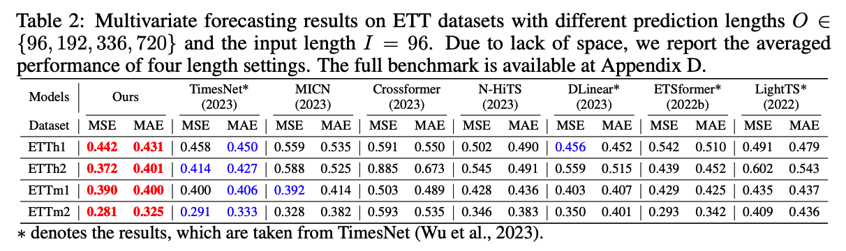
c) Extension to Multivariate TSF

(2) Model Analysis

a) Temporal Locality and Globality: Figure 6(a)

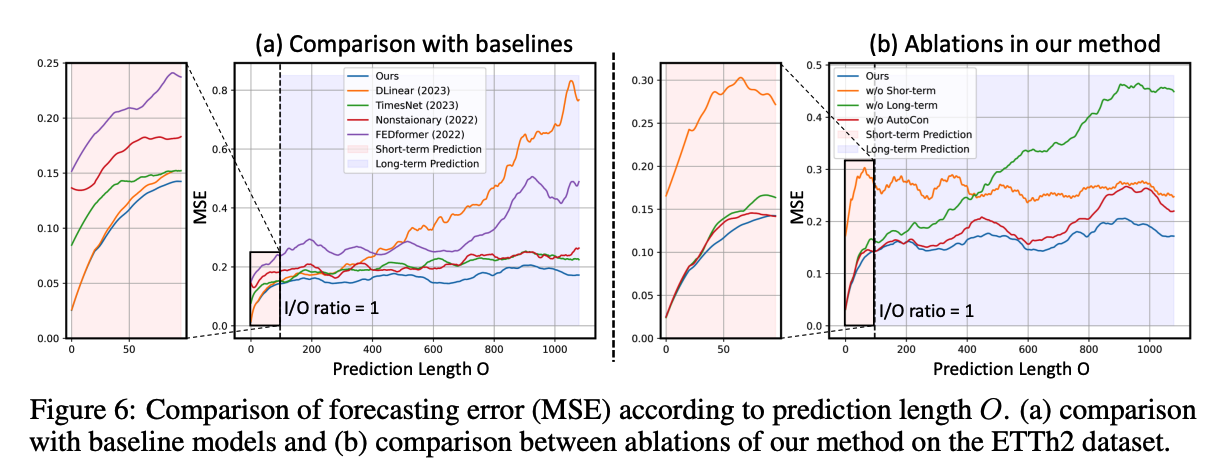
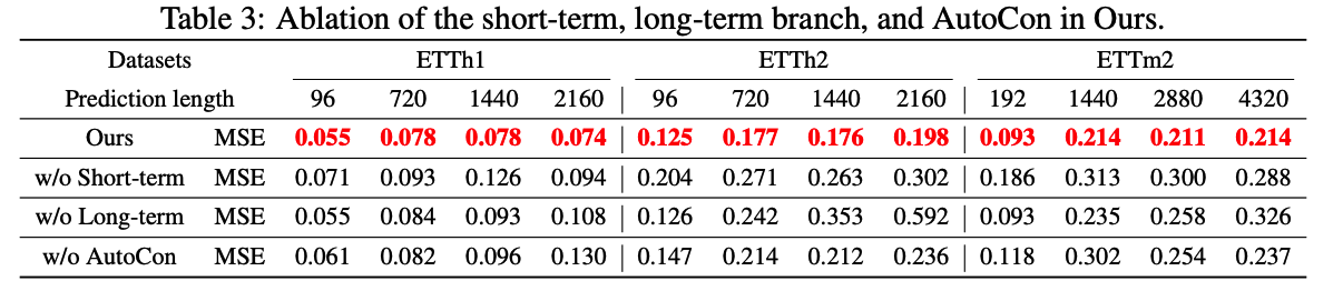
b) Ablation Studies: Figure 6(b), Table 3

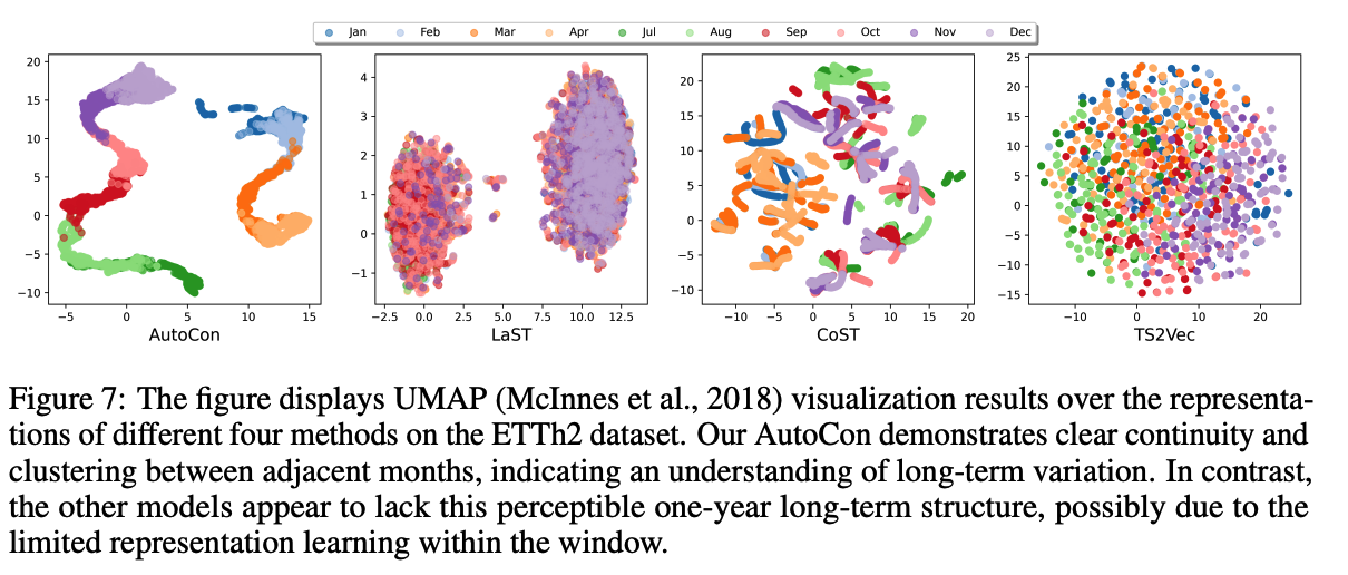
(3) Comparison with Representation Learning methods

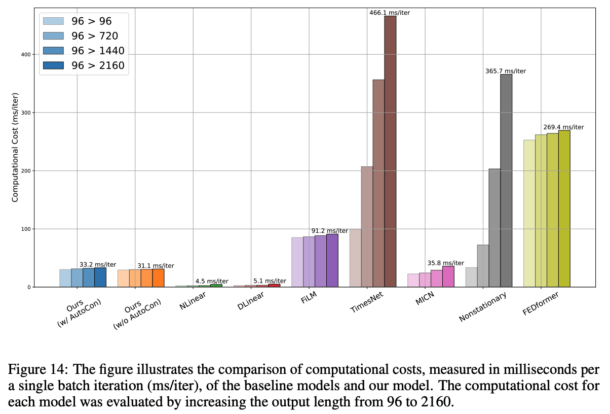
(4) Computational Efficiency Comparison

( Dataset: ETT dataset )

• w/o AutoCon : computational times of 31.1 ms/iter

  ( second best after the linear models )

• w/o AutoCon : does not increase significantly (33.2 ms/iter)
  • \(\because\) No augmentation process and the autocorrelation calculation occurs only once during the entire training.
• Transformer-based models (Nonstationary 365.7 ms/iter)
• state-of-the-art CNN-based models (TimesNet 466.1 ms/iter)