(paper) Learning Discrete Structures for GNNs

Learning Discrete Structures for GNNs (2019, 145)

Contents

1. Abstract
2. Introduction
3. Background
   1. Graph Theory Basics
   2. GNNs
   3. Bilevel Programming in ML
4. Learning Discrete Graph Structures
   1. Jointly Learning the Structure & Parameters
   2. Structure Learning via Hypergradient Descent

0. Abstract

GNN

• incorporate a spare & discrete dependency structure between data
• but can be used with “GRAPH-structure” data
  • however, most of them are noisy & incomplete

propose to “jointly” learn the

• 1) graph structure
• 2) parameters of GCNs

by approximately solving a “bilevel program”, that learns a discrete probability distribution on the edges of the graph

1. Introduction

while graph structure is available in some domains,

if not…has to be ‘inferred or constructed’!

Possible approach

• 1) create kNN graph ( based on some similarity measure )
  • shortcomings :
    • 1) choice of \(k\)?
    • 2) choice of ‘similarity measure’?
• 2) kernel matrix to model similarity
  • at the cost of dense dependency structure
• 3) this paper…

Proposal

• Goal
  • 1) learning “discrete” & “sparse” dependencies between data,
  • 2) while simultaneously training the “parameters of GCN”
• Model
  • generative probabilistic model for graphs
  • edges : random variables
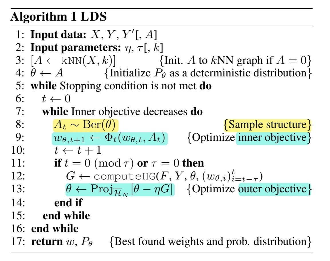
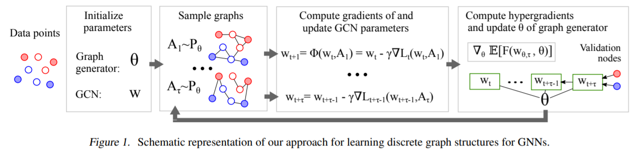
• Procedure
  • **(step 1) sample the structure **
    • ( by minimizing inner objective )
    • training error
  • (step 2) optimize the edge distn parameters
    • ( by minimizing outerobjective )
    • validation error

2. Background

(1) Graph Theory Basics

Notation

• graph \(G\) : pair \((V, E)\)
  • nodes : \(V=\left\{v_{1}, \ldots, v_{N}\right\}\)
  • edges : \(E \subseteq V \times V\)
• \(N\) : # of nodes
• \(M\) : # of edges
• graph Laplacian : \(L=D-A\)
  • \(D_{i, i}=\sum_{j} A_{i, j}\),
  • \(D_{i, j}=0\) if \(i \neq j\)

(2) GNNs

will focus especially on GCNs

GNN’s 2 inputs

• 1) feature matrix \(X \in \mathcal{X}_{N} \subset \mathbb{R}^{N \times n}\)
  • \(n\) : # of different node features
• 2) graph \(G=(V, E)\)
  • with adjacency matrix \(A \in \mathcal{H}_{N}\)

Notation

• class labels : \(\mathcal{Y}\)

• labeling function : \(y: V \rightarrow \mathcal{Y}\)

Objective :

• given a set of training nodes \(V_{\text {Train }}\) ….
• learn a function \(f_{w}: \mathcal{X}_{N} \times \mathcal{H}_{N} \rightarrow \mathcal{Y}^{N}\)
• \[L(w, A)=\sum_{v \in V_{\text {Train }}} \ell\left(f_{w}(X, A)_{v}, y_{v}\right)+\Omega(w),\]

\(\rightarrow\) “INNER optimization” / “GCN parameters”

Example of \(f_w\) : “2 hidden layer GCN”

• compute class probabilities as…

  \(f_{w}(X, A)=\operatorname{Softmax}\left(\hat{A} \operatorname{ReLu}\left(\hat{A} X W_{1}\right) W_{2}\right)\).

  • \(w=\left(W_{1}, W_{2}\right)\) : parameters of GCN

  • \(\hat{A}\) : normalized adjacency matrix

    ( = \(\tilde{D}^{-1 / 2}(A+I) \tilde{D}^{-1 / 2}\) , where \(\tilde{D}_{i i}=1+\sum_{j} A_{i j} .\) )

(3) Bilevel Programming in ML

Optimization problems, constrained with another optimization problem

\(\min _{\theta, w_{\theta}} F\left(w_{\theta}, \theta\right)\) such that \(w_{\theta} \in \arg \min _{w} L(w, \theta)\).

2 objective functions

• \(F\) : outer objective
• \(L\) : inner objective

3. Learning Discrete Graph Structures

setting : challenging scenarios…where

• graph structures is “missing” / “incomplete” / “noisy”
• variables
  • inner variables = parameters of GCN
  • outer variables = parameters of generative probabilistic model for graphs

(1) Jointly Learning the Structure & Parameters

assume a known target \(V_{val}\) ( validation dataset )

\(\rightarrow\) can estimate “generalization error”

[ OUTER = parameter of graph structure ]

Find \(A \in \mathcal{H}_{N}\), which minimizes the function

• \(F\left(w_{A}, A\right)=\sum_{v \in V_{\mathrm{val}}} \ell\left(f_{w_{A}}(X, A)_{v}, y_{v}\right)\).
• since discrete….
  • propose to model each edge with “Bernoulli r.v”

[ INNER = parameters of GCN ]

• \(L(w, A)=\sum_{v \in V_{\text {Train }}} \ell\left(f_{w}(X, A)_{v}, y_{v}\right)+\Omega(w)\).

Reformulation

\[\begin{gathered} \min _{\theta \in \overline{\mathcal{H}}_{N}} \mathbb{E}_{A \sim \operatorname{Ber}(\theta)}\left[F\left(w_{\theta}, A\right)\right] \\ \text { such that } w_{\theta}=\arg \min _{w} \mathbb{E}_{A \sim \operatorname{Ber}(\theta)}[L(w, A)] \end{gathered}\]

Expected output of GCN

• (original)

  \(f_{w}^{\exp }(X)=\mathbb{E}_{A}\left[f_{w}(X, A)\right]=\sum_{A \in \mathcal{H}_{N}} P_{\theta}(A) f_{w}(X, A)\).

• (empirical estimate)

  \(\hat{f}_{w}(X)=\frac{1}{S} \sum_{i=1}^{S} f_{w}\left(X, A_{i}\right),\).

  • \(S\) : # of samples to draw
  • sample \(S\) graphs from distn \(P_{\theta}\)

(2) Structure Learning via Hypergradient Descent

Variables

• Outer : \(\theta\)
• Inner : \(w\)

[ INNER ]

\(\mathbb{E}_{A \sim \operatorname{Ber}(\theta)}[L(w, A)]=\sum_{A \in \mathcal{H}_{N}} P_{\theta}(A) L(w, A)\).

• composed of sum of \(2^{N^2}\) terms
• intractable! use SGD
  • \(w_{\theta, t+1}=\Phi\left(w_{\theta, t}, A_{t}\right)=w_{\theta, t}-\gamma_{t} \nabla L\left(w_{\theta, t}, A_{t}\right)\).
  • where \(A_t \sim \text{Ber}(\theta)\)

[ OUTER ]

• \(w_{\theta, T}\) : approximate minimizer of \(\mathbb{E}[L]\)
• need an estimator for hypergradient, \(\nabla_{\theta} \mathbb{E}_{A \sim \operatorname{Ber}(\theta)}\left[F\left(w_{\theta, T}, A\right)\right] .\)
• Trick
  • smooth reparameterization for \(P_{\theta}\)
  • (before) \(z \sim P_{\theta}\)
  • (after) \(z=\operatorname{sp}(\theta, \varepsilon)\) for \(\varepsilon \sim P_{\varepsilon}\)
• \(\nabla_{\theta} \mathbb{E}_{z \sim P_{\theta}}[h(z)]=\mathbb{E}_{\varepsilon \sim P_{\varepsilon}}\left[\nabla_{\theta} h(\operatorname{sp}(\theta, \varepsilon))\right]= \mathbb{E}_{z \sim P_{\theta}}\left[\nabla_{z} h(z) \nabla_{\theta} z\right]\).
• use Identity Mapping \(A = \operatorname{sp}(\theta, \varepsilon) = \theta\)
  • \(\nabla_{\theta} \mathbb{E}_{A \sim \operatorname{Ber}(\theta)}\left[F\left(w_{\theta, T}, A\right)\right] \approx \mathbb{E}_{A \sim \operatorname{Ber}(\theta)}\left[\nabla_{A} F\left(w_{\theta, T}, A\right)\right]\).

(3) Summary