
Distribution Shift (Data Shift, DS)
1. Data shift
-
Training distribution \(\neq\) Test distribution
( \(\mathrm{P}_{\mathrm{tra}}(\mathrm{y}, \mathrm{x}) \neq \mathrm{P}_{\mathrm{tst}}(\mathrm{y}, \mathrm{x})\) )
-
다른 표현: concept shift, concept drift
2. Categories of DS
아래의 2가지에 따라, 총 4가지로 구분
-
(1) “X의 분포”가 변화했는가? …. \(\mathrm{P}(x)\)
-
(2) “Y의 분포”가 변화했는가? …. \(\mathrm{P}(y)\)
-
(3) “X \(\rightarrow\) Y 의 관계”가 변화했는가? …. \(\mathrm{P}(y \mid x)\)
-
(4) “Y \(\rightarrow\) X 의 관계”가 변화했는가? …. \(\mathrm{P}(x \mid y)\)
(1) Covariate shift
( 한 줄 요약: X의 분포가 달라졌다 )
-
(1) X: 다르다 ( \(P_{\text {tra }}(x)\) \(\neq \mathrm{P}_{\text {tst }}(\mathrm{x})\) )
-
(2) Y: -
-
(3) X \(\rightarrow\) Y: 같다 ( \(\mathrm{P}_{\text {tra }}(y \mid x)=P_{\text {tst }}(y \mid x)\) )
-
(4) Y \(\rightarrow\) X: -
(2) Prior probability shift
( 한 줄 요약: Y의 분포가 달라졌다 )
- (1) X: -
- (2) Y: 다르다 ( \(P_{\text {tra }}(y)\) \(\neq \mathrm{P}_{\text {tst }}(\mathrm{y})\) )
- (3) X \(\rightarrow\) Y: -
- (4) Y \(\rightarrow\) X: 같다 ( \(\mathrm{P}_{\text {tra }}(x \mid y)=P_{\text {tst }}(x \mid y)\) )
(3) Concept shift
( 한 줄 요약: X & Y의 관계가 달라졌다 )
- (1) X: 같다 ( \(P_{\text {tra }}(x)\) \(= \mathrm{P}_{\text {tst }}(\mathrm{x})\) )
- (2) Y: 같다 ( \(P_{\text {tra }}(y)\) \(= \mathrm{P}_{\text {tst }}(\mathrm{y})\) )
- (3) X \(\rightarrow\) Y: 다르다 ( \(\mathrm{P}_{\text {tra }}(y \mid x) \neq P_{\text {tst }}(y \mid x)\) )
- (4) Y \(\rightarrow\) X: 다르다 ( \(\mathrm{P}_{\text {tra }}(x \mid y) \neq P_{\text {tst }}(x \mid y)\) )
(4) Internal covariate shift
- DL에서 layer가 입력받는 분포가 다를 경우, 불안정한 학습
- (현재 Out of scope)
3. Major Causes of DS
2가지 주요 원인
- (1) Sampling bias
- 편향된 방법을 통해 train data를 획득 하는 경우
- (2) Non-stationary environment
- 시/공간적인 이유로, 변화가 발생
4. Identifying DS
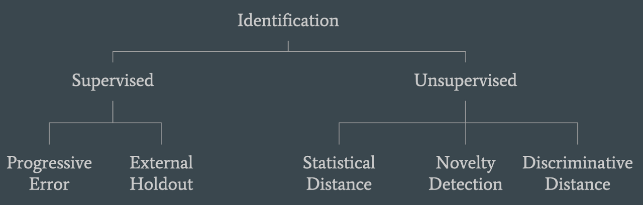
2가지 주요 방법
- (1) Statistical distance
- (2) Novelty detection
- (3) Discriminative Distance
(1) Statistical distance
- When? 시간에 따라 분포가 변화하는 경우
- How? 히스토그램
- Example:
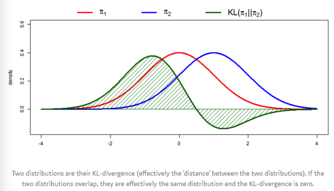
Diverse metrics
- (1) Population Stability Index (PSI)
- (2) Kolmogorov-Smirnov statistic
- (3) Kullback-Lebler divergence (or other f-divergences)
- (4) Histogram intersection.
한계점: High-dimensional data
(2) Novelty detection
Procedure
- Step 1) Source distribution을 모델링
- Step 2) 새로운 데이터가 왔을 때, 해당 distribution에서의 probability 계산
- if low \(\rightarrow\) novelty!
- ex) One-class SVM
High-dimensional data에 좋지만, (1) Statistical distance만큼 효과적이지는 X
(3) Discriminative Distance
핵심: Discriminator (or classifier)를 학습해서, 해당 데이터의 출처 ( source or target )을 파악하자
마찬가지로 High-dimensional data에 좋지만, (1) Statistical distance만큼 효과적이지는 X
5. Handling DS
한 줄 요약: Dataset을 보정/수정함으로써 해결하자!
(1) Feature Removal
- Statistical distance를 통해 shift의 정도 측정 가능!
- 특정 변수 제거 시, statistical distance가 얼마나 바뀌는지를 통해 제거 여부 판단 ( with 특정 threshold ) \(\rightarrow\) Train & Test 에서의 값이 만힝 상이하지만, 예측력 향상에 도움 안되는 변수는 버리기!
(2) Importance Reweighting
한 줄 요약: Test 데이터와 유사한 Train 데이터가 더 중요하므로, 가중치를 보다 높게 주기!
References
https://data-newbie.tistory.com/357?category=781224