(paper) Challenges and Approaches to Time-Series Forecasting in DT Center Telemetry ; A Survey

Challenges and Approaches to Time-Series Forecasting in DT Center Telemetry ; A Survey (2021)

Contents

1. Abstract
2. Introduction
3. Problem Definition & Requirements
   1. Multi-Period Forecasting
   2. Challenges in Multi-Period Forecasting
4. Forecasting Techniques
   1. SSM (State Space Models)
   2. EWMA (Exponential Weighted Moving Average)
   3. GARCH (Generalized Autoregressive Conditional Heteroskedastic Model)
   4. Specialized Libraries
   5. Deep Learning models
   6. Probabilistic Models

0. Abstract

summarize & evaluate performance of well-known time series forecasting techniques

1. Introduction

• section 2 : problem definition, requirements & forecasting models’ assumption
• section 3 : widely used time series based forecasting techniques
• section 4 : experiment
• section 5 : conclude the outcome

2. Problem Definition & Requirements

\(k\) factors of time series : \(T_{o}, T_{1}, . . T_{k}\)

\(\rightarrow\) determine the response variable \(y_{0}, y_{1}, \ldots, y_{n}\)

Two Problems

• 1) Single (Next) Period Prediction

  \(y_{n+1}=f\left(T_{0}, T_{1},, T_{k} ; y_{0}, y_{1}, \ldots, y_{n}\right)\).

• 2) Multi Period Prediction

  \(y_{n+1, n+2, \ldots n+m}=f\left(T_{0}, T_{1},, T_{k} ; y_{0}, y_{1}, \ldots, y_{n}\right)\).

(1) Multi-Period Forecasting

( = 예측 대상 시점이 “여러 시점” )

Various Approaches

• 1) fixed-length forecast
  • based on training data
  • does not expose its internal state after forecasting
• 2) arbitrary-length forecast
  • output as a function of time .
• 3) single-point rolling prediction
  • exposes internal state, allowing for updating it with the prediction
• 4) fixed multiple-point rolling prediction
  • performed in batches

(2) Challenges in Multi-Period Forecasting

\(y_{n+1, n+2, \ldots n+m}=f\left(T_{0}, T_{1},, T_{k} ; y_{0}, y_{1}, \ldots, y_{n}\right)\).

위 식에서, \(y_{n+2}\) 예측 시, \(y_{n+1}\) 을 모른다는 사실!

이를 풀기 위한 노력들 ex) :

consistent treatment in modeling phase

• ex) LSTM : built-in capacity for multi-period forecasting

  ( but, number of future periods should be specified )

Unified arbitrary-length prediction generator

stepwise method

• 1) predict a single datapoint
• 2) feeding it back into prediction model

3. Forecasting Techniques

(1) SSM (State Space Models)

a) ARIMA (Autoregressive Integrated Moving Average)

• most widely used statistical model
• characterized by 3 factors : ARIMA(p,d,q)
  • \(p\) : order ( # of time lags ) of auto-regressive component
  • \(d\) : degree of differencing
  • \(q\) : order of moving average model

Multivariate Extensions to ARIMA

• VARMA ( = VAR = Vector Autoregressive Models ) :

  set of dependent variables with a regression for each one

• ARIMAX :

  set of independent variables (exogenous) for a single dependent variable

(2) EWMA (Exponential Weighted Moving Average)

only consider one period forecast

simple EWMA :

• \(y_{t+1}=\alpha y_{t}+(1-\alpha) y_{t-1}\).
  • \(y_{0}=y_{0}\).
  • where, \(y_{t+1}\) is the forecast at \(y_{t}\).

Holt’s Extension : incorporate slope/trend in EWMA

\(y_{t+1}=l_{t}+y_{t-1}\).

• \(l_{t}=\alpha y_{t}+(1-\alpha)\left(l_{t-1}+b_{t-1}\right)\).
  • \(b_{t}=\beta\left(b_{t}-s_{t-1}\right)+(1-\beta) b_{t-1}\).

Holt-Winter extension : extension of Holt’s ( + additional term for seasonality )

\(y_{t+1}=l_{t}+b_{t}+s_{t}\).

• \(l_{t}=\alpha y_{t}+(1-\alpha)\left(l_{t-1}+b_{t-1}\right)\).
• \(b_{t}=\beta\left(l_{t}-l_{t-1}\right)+(1-\beta) b_{t-1}\).
• \(s_{t}=\gamma\left(y_{t}-l_{t}\right)+(1-\gamma) s_{t-1}\).

(3) GARCH (Generalized Autoregressive Conditional Heteroskedastic Model)

supports heteroskedastic process

• [AR = autoregressive] regressed function of time series
• [C = conditional] forecast for next time : condition in current time period
• [H = heteroskedastic] variance is not constant

a) STD (Seasonal Trend Decomposition) Predictor

extension of LR that incorporates seasonal trends

• LR : based on time series
• seasonality : modeled by transforming time/holidays into categorical features

[ Equation ]

\(\hat{y}_{t}=L R(t)+L R\left(F_{\text {time }}(t)\right)\).

• \(L R\) : standard LR
• \(F_{\text {time }}(t)\) : categorical features based on time

b) STAR (Seasonal Trend Autoregressive) Predictor

extends the STD model by incorporating an autoregressive component

[ Equation ]

\(\hat{y}_{t}=L R(t)+L R\left(F_{\text {time }}(t)\right)+L R\left(y_{t-a w: t}\right)\).

• \(LR\) : standard LR
• \(F_{\text {time }}(t)\) : categorical features based on time
• \(aw\) : autoregression window

(4) Specialized Libraries

a) FB (Facebook) Prophet

• 생략

b) GluonTS

• 생략

(5) Deep Learning models

생략

• RNN
• LSTM
• Bi-LSTM

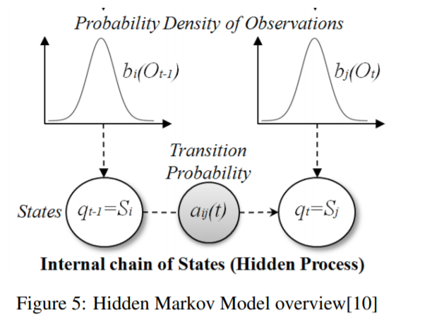
(6) Probabilistic Models

learn parameters, using optimization approaches like EM algorithm

a) HMM

• based on Markov Change
• strong assumption : have dependence on ONLY current state