(paper 98) AdaRNN; Adaptive Learning and Forecasting for Time Series

AdaRNN: Adaptive Learning and Forecasting for Time Series (CIKM 2021)

https://arxiv.org/pdf/2108.04443.pdf

https://github.com/jindongwang/transferlearning/tree/master/code/deep/adarnn

Contents

1. Abstract
2. Introduction
3. Related Work
   1. TS analysis
   2. Distribution matching
4. Problem Formulation
5. AdaRNN
   1. Temporal Distribution Characterization (TDC)
   2. Temporal Distribution Matching (TDM)

Abstract

Distribution shift

• statistical properties of a TS can vary with time

Formulate the Temporal Covariate Shift (TCS) problem for TSF

Adaptive RNNs (AdaRNN)

AdaRNN is sequentially composed of 2 modules

• (1) Temporal Distribution Characterization
  • aims to better characterize the distribution information in a TS
• (2) Temporal Distribution Matching
  • aims to reduce the distribution mismatch in the TS

Summary : general framework with flexible distribution distances integrated.

1. Introduction

Non-stationary TS

• Statistical properties of TS are changing over time

• ex) Figure 1

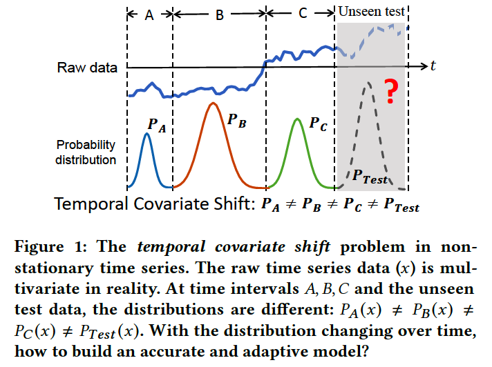
HOWEVER … \(P(y \mid x)\) is usually considered to be unchanged!

Two main challenges of the problem

1. How to characterize the distribution in the data to maximally harness the common knowledge in these varied distributions?
2. How to invent an RNN-based distribution matching algorithm to maximally reduce their distribution divergence while capturing the temporal dependency?

AdaRNN

• a novel framework to learn an accurate and adaptive prediction model.
• composed of two modules.
  • (1) temporal distribution characterization (TDC)
    • split the training data into 𝐾 most diverse periods that are with large distribution gap inspired by the principle of maximum entropy
  • (2) temporal distribution matching (TDM)
    • dynamically reduce distribution divergence using RNN

2. Related Work

(1) TS analysis

• pass

(2) Distribution Matching

Domain adaptation (DA)

• bridge the distribution gap
• often performs instance re-weighting or feature transfer to reduce the distribution divergence in training and test data
• ex) domain-invariant representations can be learned

Domain generalization (DG)

• also learns a domain-invariant model on multiple source domains

DA vs. DG

• DA : test data is ACCESSIBLE
• DG : test data is NOT ACCESSIBLE

3. Problem Formulation

[Problem 1] \(r\)-step ahead prediction

Notation

• \(\mathcal{D}=\left\{\mathbf{x}_i, \mathbf{y}_i\right\}_{i=1}^n\).
  • \(n\) : number of TS
  • where \(\mathbf{x}_i=\left\{x_i^1, \cdots, x_i^{m_i}\right\} \in \mathbb{R}^{p \times m_i}\)
    • \(m_i\) : length of \(i\)-th TS
    • \(p\) : number of channels
  • where \(\mathbf{y}_i=\left(y_i^1, \ldots, y_i^c\right) \in \mathbb{R}^c\)

[Learn] model \(\mathcal{M}: \mathrm{x}_i \rightarrow \mathrm{y}_i\)

• predict future \(r \in \mathbb{N}^{+}\)steps for segments \(\left\{\mathbf{x}_j\right\}_{j=n+1}^{n+r}\)

• Previous works : all time series segments, \(\left\{\mathbf{x}_i\right\}_{i=1}^{n+r}\), are assumed to follow the same data distribution

Covariate Shift

Notation:

• train distn : \(P_{\text {train }}(\mathrm{x}, y)\)
• test distn : \(P_{\text {test }}(\mathrm{x}, y)\)

Definition of Covariate Shift

• (1) marginal probability distributions are different ( \(P_{\text {train }}(\mathbf{x}) \neq P_{\text {test }}(\mathbf{x})\) )
• (2) conditional distributions are the same ( \(P_{\text {train }}(y \mid \mathbf{x})=P_{\text {test }}(y \mid \mathbf{x})\) )

\(\rightarrow\) for NON-TS data

( TS data : Temporal Covariate Shift )

Temporal Covariate Shift (TCS)

Notation

• time series data \(\mathcal{D}\) with \(n\) labeled segments
• can be split into \(K\) periods
  • i.e., \(\mathcal{D}=\left\{\mathcal{D}_1, \cdots, \mathcal{D}_K\right\}\), where \(\mathcal{D}_k=\left\{\mathrm{x}_i, \mathrm{y}_i\right\}_{i=n_k+1}^{n_{k+1}}\), \(n_1=0\) and \(n_{k+1}=n\).

Definition of Temporal Covariate Shift

• (2) all the segments in the same period \(i\) follow the same data distribution ( \(P_{\mathcal{D}_i}(\mathbf{x}, y)\) )
• (2) for different time periods \(1 \leq i \neq j \leq K\), \(P_{\mathcal{D}_i}(\mathbf{x}) \neq P_{\mathcal{D}_j}(\mathbf{x})\) and \(P_{\mathcal{D}_i}(y \mid \mathbf{x})=P_{\mathcal{D}_j}(y \mid \mathbf{x})\).

Key point: Capture the common knowledge shared among different periods of \(\mathcal{D}\)

• number of periods \(K\) and the boundaries of each period under TCS are usually unknown in practice
• need to first discover the periods by comparing their underlying data distributions such that segments in the same period follow the same data distributions.

[Problem 1] \(r\)-step ahead prediction under TCS

Given \(\mathcal{D}=\left\{\mathbf{x}_i, \mathrm{y}_i\right\}_{i=1}^n\) for training.

\(P_{\mathcal{D}_i}(\mathrm{x}, y)\) while for different time periods \(1 \leq i \neq j \leq K, P_{\mathcal{D}_i}(\mathbf{x}) \neq P_{\mathcal{D}_j}(\mathbf{x})\) and \(P_{\mathcal{D}_i}(y \mid \mathbf{x})=P_{\mathcal{D}_j}(y \mid \mathbf{x})\).

Goal:

• automatically discover the \(K\) periods in the training TS data
• learn a prediction model \(\mathcal{M}: \mathbf{x}_i \rightarrow \mathrm{y}_i\) by exploiting the commonality among different time periods, such that it makes precise predictions on the future r segments, \(\mathcal{D}_{t s t}=\left\{\mathrm{x}_j\right\}_{j=n+1}^{n+r}\).

Assumption: Test segments are in the same time period

• \(P_{\mathcal{D}_{t s t}}(\mathbf{x}) \neq P_{\mathcal{D}_i}(\mathbf{x})\) and \(P_{\mathcal{D}_{t s t}}(y \mid \mathbf{x})=P_{\mathcal{D}_i}(y \mid \mathbf{x})\) for any \(1 \leq i \leq K\).

4. AdaRNN

Consists of 2 novel algorithms ; TDC & TDM

Procedure

• step 1) use TDC to split into periods
  • which fully characterize its distn information
• step 2) apply TDM to perform distribution matching among periods
  • build a prediction model \(\mathcal{M}\)

Rationale behind AdaRNN

• [TDC] \(\mathcal{M}\) is expected to work under the WORST distn scenarios, where distn gaps are large
• [TDM] use the common knowledge of the learend time periods
  • by matching their distns via RNNs

(1) Temporal Distribution Characterization (TDC)

Splitting the TS by solving an optimization problem

\(\begin{aligned} & \max _{0<K \leq K_0} \max _{n_1, \cdots, n_K} \frac{1}{K} \sum_{1 \leq i \neq j \leq K} d\left(\mathcal{D}_i, \mathcal{D}_j\right) \\ & \text { s.t. } \forall i, \Delta_1< \mid \mathcal{D}_i \mid <\Delta_2 ; \sum_i \mid \mathcal{D}_i \mid =n \end{aligned}\).

• \(d\) is a distance metric
• \(\Delta_1\) and \(\Delta_2\) are predefined parameters to avoid trivial solutions
• \(K_0\) is the hyperparameter to avoid over-splitting

(2) Temporal Distribution Matching (TDM)

learn the common knowledge shared by different periods

• via matching their distributions

\(\rightarrow\) \(\mathcal{M}\) is expected to generalize well on unseen test data

\(\mathcal{L}_{\text {pred }}(\theta)=\frac{1}{K} \sum_{j=1}^K \frac{1}{ \mid \mathcal{D}_j \mid } \sum_{i=1}^{ \mid \mathcal{D}_j \mid } \ell\left(\mathbf{y}_i^j, \mathcal{M}\left(\mathbf{x}_i^j ; \theta\right)\right)\).

• where \(\left(\mathrm{x}_i^j, \mathrm{y}_i^j\right)\) denotes the \(i\)-th labeled segment from period \(\mathcal{D}_j\)

Distribution matching is usually performed on high-level representations

• on the final outputs of the cell of RNN models

  ( use \(\mathbf{H}=\left\{\mathbf{h}^t\right\}_{t=1}^V \in \mathbb{R}^{V \times q}\) to denote the \(V\) hidden states of an RNN with feature dimension \(q\). )

Period-wise distribution matching

• on the final hidden states for a pair \(\left(\mathcal{D}_i, \mathcal{D}_j\right)\)

\(\mathcal{L}_{d m}\left(\mathcal{D}_i, \mathcal{D}_j ; \theta\right)=d\left(\mathbf{h}_i^V, \mathbf{h}_j^V ; \theta\right)\).