(paper) Modeling Long and Short Term Temporal Patterns with DNN

Modeling Long and Short Term Temporal Patterns with DNN (2017, 496)

Contents

1. Abstract
2. Introduction
3. Related Background
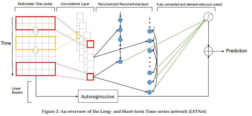
4. Framework
   1. Problem Formulation
   2. Convolutional Component
   3. Recurrent Component
   4. Recurrent Skip Component
   5. Dense Layer
   6. Temporal Attention Layer
   7. Autoregressive Component
   8. Loss Function

0. Abstract

• goal : MTS forecasting

• Temporal data = mixture of long & short term patterns
  • traditional models ( GP, AR ) fails..
• propose LSTNet (Long and Short-term Time-series Network)

LSTNet

(1) use CNN & RNN to extract …

• 1) short term local dependency patterns ( among variables )
• 2) long term patterns for time series trends

(2) leverage traditional autoregressive model to tackle the scale insensitive problem

1. Introduction

MTS key point :

• how to capture & leverage “dynamics dependencies among multiple variables”

Real-world data :

• mixture of LONG & SHORT term repeating patterns
• how to capture both?

LSTNet ( Long and Short-term Time-series Network )

• 1) CNN
  • to discover “LOCAL dependency patterns” among multi-dimensional input
• 2) RNN
  • to capture “complex LONG term dependencies”
• 3) Recurrent-skip
  • capture very long-term dependence patterns
• 4) incorporate a traditional autoregressive linear model in parallel

2. Related Background

Univariate TS

• ARIMA ( Box-Jenkins methodology )

  \(\rightarrow\) rarely used in high-dimensional MTS ( \(\because\) high computational cost )

• VAR ( Vector Autoregression )

  • VAR = AR + MTS
  • widely used MTS for its simplicity

  • ignores the dependencies between output variables

  • model capacity of VAR grows ….

    • linearly over the temporal window size

    • quadratically over the number of variables

Others

• SVR : non-linear

• Ridge, LASSO …. : linear

  \(\rightarrow\) practically more efficient for MTS, but fail to capture complex relationship

• GP (Gaussian Process) : non-parametric

  • can be applied to MTS
  • can be used as a prior over the function space in Bayesian Inference
  • high computation complexity

3. Framework

(1) Problem Formulation

interested in MTS

Notation :

• \(Y=\left\{\boldsymbol{y}_{1}, \boldsymbol{y}_{2}, \ldots, \boldsymbol{y}_{T}\right\}\) : fully observed TS
  • \(\boldsymbol{y}_{t} \in \mathbb{R}^{n}\) ( \(n\) : # of variables )
• [INPUT] \(X_{T}=\left\{\boldsymbol{y}_{1}, \boldsymbol{y}_{2}, \ldots, \boldsymbol{y}_{T}\right\} \in \mathbb{R}^{n \times T}\).
• [OUTPUT] \(\hat{\boldsymbol{y}}_{T+h+1}\)

(2) Convolutional Component

[FIRST layer]

• CNN without pooling
• goal : extract SHORT term patterns & LOCAL dependencies between variables

(3) Recurrent Component

[SECOND layer]

• output of CNN is fed into “Recurrent component” & “Recurrent-skip component”

\(\begin{aligned} r_{t} &=\sigma\left(x_{t} W_{x r}+h_{t-1} W_{h r}+b_{r}\right) \\ u_{t} &=\sigma\left(x_{t} W_{x u}+h_{t-1} W_{h u}+b_{u}\right) \\ c_{t} &=R E L U\left(x_{t} W_{x c}+r_{t} \odot\left(h_{t-1} W_{h c}\right)+b_{c}\right) \\ h_{t} &=\left(1-u_{t}\right) \odot h_{t-1}+u_{t} \odot c_{t} \end{aligned}\).

(4) Recurrent-skip Component

• to solve gradient vanishing problem

\(\begin{aligned} &r_{t}=\sigma\left(x_{t} W_{x r}+h_{t-p} W_{h r}+b_{r}\right) \\ &u_{t}=\sigma\left(x_{t} W_{x u}+h_{t-p} W_{h u}+b_{u}\right) \\ &c_{t}=R E L U\left(x_{t} W_{x c}+r_{t} \odot\left(h_{t-p} W_{h c}\right)+b_{c}\right) \\ &h_{t}=\left(1-u_{t}\right) \odot h_{t-p}+u_{t} \odot c_{t} \end{aligned}\).

• \(p\) : number of hidden cells skipped

(5) Dense Layer

combine outputs of

• 1) Recurrent components ( \(h_t^R\) )
• 2) Recurrent-skip components ( \(h_t^S\) )

output of dense layer :

• \(h_{t}^{D}=W^{R} h_{t}^{R}+\sum_{i=0}^{p-1} W_{i}^{S} h_{t-i}^{S}+b\).

(6) Temporal Attention Layer

Recurrent skip layer : needs “pre-defined hyperparameter \(p\)”

\(\rightarrow\) use attention instead! ( to make weighted combinations )

\(\boldsymbol{\alpha}_{t}=\operatorname{AttnScore}\left(H_{t}^{R}, h_{t-1}^{R}\right)\).

• attention weight \(\boldsymbol{\alpha}_{t} \in \mathbb{R}^{q}\)

• \(H_{t}^{R}=\left[h_{t-q}^{R}, \ldots, h_{t-1}^{R}\right]\) is a matrix stacking the hidden representation of RNN column-wisely

• \(\text{AttnScore}\) : similarity functions

  ex) dot product, cosine, or parameterized by a simple multi-layer perceptron…

Weighted Context vector : \(c_{t}=H_{t} \alpha_{t}\).

Final : \(h_{t}^{D}=W\left[c_{t} ; h_{t-1}^{R}\right]+b\).

(7) Autoregressive Component

capture non-linearity by “CNN” & “RNN”

\(\rightarrow\) but…. scale of output is not sensitive to scale of inputs!

Solution : decompose the final prediction of LSTNet into a…

• 1) linear part : to deal with local scaling issue ( \(h_{t}^{L}\) )
  • use AR model for this!
  • \(h_{t, i}^{L}=\sum_{k=0}^{q^{a r}-1} W_{k}^{a r} \boldsymbol{y}_{t-k, i}+b^{a r}\).
• 2) non-linear part : containing recurring patterns ( \(h_{t}^{D}\) )

Final Prediction : \(\hat{Y}_{t}=h_{t}^{D}+h_{t}^{L}\)

(8) Loss Function

\(\underset{\Theta}{\operatorname{minimize}} \sum_{t \in \Omega_{\text {Train }}} \mid \mid Y_{t}-\hat{Y}_{t-h}\mid \mid_{F}^{2}\).