(paper) Deep State Space Models for TS Forecasting

Deep State Space Models for TS Forecasting (2018,266)

Contents

1. Abstract
2. Introduction
3. Related Work
4. Background
5. DSSM (Deep State Space Models)

Abstract

characteristic of DSSM

• probabilistic TSF model

• SSM + Deep Learning (RNN)
• pros)
  • SSM : data efficiency & interpretability
  • RNN : learn complex patterns

1. Introduction

(1) State Space models

• framework for modeling/learning time series patterns ( ex. trend, seasonality )

• ex) ARIMA, exponential smoothing

• well suited, when “structure of TS is weel understood”

• pros & cons

  • pros : (1) interpretability + (2) data efficiency
  • cons : requires TS with LONG history

• traditional SSMs cannot infer shared patterns for similar TSs

  ( fitted separately )

(2) DNN

• pass

(3) DSSM

• bridge the gap between those two ( SSM + RNN )

• parameters of RNN are learned “jointly”,

  using “TS” & “covariates”

• interpretable!

2. Related Work

combining SSM & RNNs

• DMM (Deep Markov Model)
  • keeps Gaussian transition dynamics with mean/cov matrix parameterized by MLP
• Stochastic RNNs
• Variational RNNs
• Latent LSTM Allocation
• State-Space LSTM

Most relevant to this work is … “KVAE” (Kalman VAE)

• keep the linear Gaussian transition structure intact

3. Background

(1) Basics

Notation

• \(N\) univariate TS : \(\left\{z_{1: T_{i}}^{(i)}\right\}_{i=1}^{N}\)
  • \(z_{1: T_{i}}^{(i)}=\left(z_{1}^{(i)}, z_{2}^{(i)}, \ldots, z_{T_{i}}^{(i)}\right)\) .
  • \(z_{t}^{(i)} \in \mathbb{R}\) : \(i\)-th time series at time \(t\)
• time-varying covariate : \(\left\{\mathbf{x}_{1: T_{i}+\tau}^{(i)}\right\}_{i=1}^{N}\)
  • \(\mathbf{x}_{t}^{(i)} \in \mathbb{R}^{D}\).

Goal : produce a set of PROBABILISTIC forecasts

• \(p\left(z_{T_{i}+1: T_{i}+\tau}^{(i)} \mid z_{1: T_{i}}^{(i)}, \mathbf{x}_{1: T_{i}+\tau}^{(i)} ; \Phi\right)\).

  • \(\Phi\) : set of learnable parameters

    ( shared between & learned jointly from ALL \(N\) time series )

  • forecast start time : \(T_{i}+1\)

  • forecast horizon : \(\tau \in \mathbb{N}_{>0}\)

  • range

    • training range : \(\left\{1,2, \ldots, T_{i}\right\}\)
    • prediction range : \(\left\{T_{i}+1, T_{i}+2, \ldots, T_{i}+\tau\right\}\)

(2) State Space Models (SSMs)

• model the “temporal structure”, via “latent state \(l_{t} \in \mathbb{R}^{L}\)“
• general SSM
  • 1) state-transition equation
    • \(p\left(\boldsymbol{l}_{t} \mid \boldsymbol{l}_{t-1}\right)\).
  • 2) observation model
    • \(p\left(z_{t} \mid \boldsymbol{l}_{t}\right)\).

Linear SSMs

• \(\boldsymbol{l}_{t}=\boldsymbol{F}_{t} \boldsymbol{l}_{t-1}+\boldsymbol{g}_{t} \varepsilon_{t}, \quad \varepsilon_{t} \sim \mathcal{N}(0,1)\).

  • \(\boldsymbol{l}_{t-1}\) : information about level/trend/seasonality
  • \(\boldsymbol{F}_{t}\) : deterministic transition matrix
  • \(\boldsymbol{g}_{t} \varepsilon_{t}\) : random innovation

• Univariate Gaussian observation model

  • \(z_{t}=y_{t}+\sigma_{t} \epsilon_{t}, \quad y_{t}=\boldsymbol{a}_{t}^{\top} \boldsymbol{l}_{t-1}+b_{t}, \quad \epsilon_{t} \sim \mathcal{N}(0,1)\).

  • initial state : isotropic Gaussian distribution

    • \(l_{0} \sim N\left(\boldsymbol{\mu}_{0}, \operatorname{diag}\left(\boldsymbol{\sigma}_{0}^{2}\right)\right)\).

(3) Parameter Learning

parameters of SSMs

• \(\Theta_{t}=\left(\boldsymbol{\mu}_{0}, \boldsymbol{\Sigma}_{0}, \boldsymbol{F}_{t}, \boldsymbol{g}_{t}, \boldsymbol{a}_{t}, b_{t}, \sigma_{t}\right), \forall t>0\).

Classical settings

• 1) dynamics are assumed to be time-invariant

  ( that is, \(\Theta_{t}=\Theta, \forall t>0\) )

• 2) if there is more than one TS, a separate set of parameters \(\Theta^{(i)}\) is learend,

  for each time series

Maximizing marginal likelihood : \(\Theta_{1: T}^{*}=\operatorname{argmax}_{\Theta_{1: T}} p_{S S}\left(z_{1: T} \mid \Theta_{1: T}\right)\)

• \(p_{S S}\left(z_{1: T} \mid \Theta_{1: T}\right):=p\left(z_{1} \mid \Theta_{1}\right) \prod_{t=2}^{T} p\left(z_{t} \mid z_{1: t-1}, \Theta_{1: t}\right)=\int p\left(\boldsymbol{l}_{0}\right)\left[\prod_{t=1}^{T} p\left(z_{t} \mid \boldsymbol{l}_{t}\right) p\left(\boldsymbol{l}_{t} \mid \boldsymbol{l}_{t-1}\right)\right] \mathrm{d} \boldsymbol{l}_{0: T}\).

4 . DSSM (Deep State Space Models)

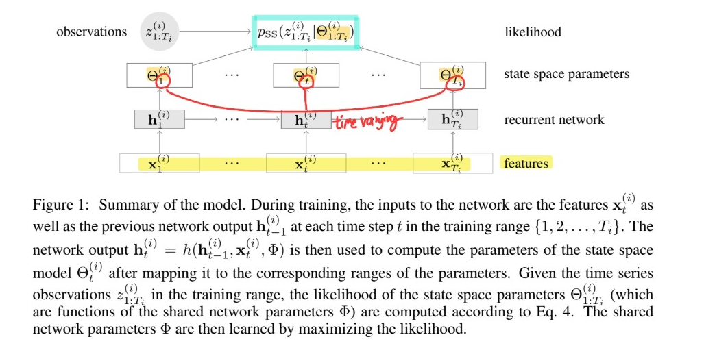
[ Step 1 ]

learns “TIME VARYING” & “GLOBAL” \(\Theta^{(i)}\)< from…

• 1) covariate vectors \(\mathbf{x}_{1:T_i}^{(i)}\).
• 2) target time series \(z_{1: T_{i}}^{(i)}\)

\[\Theta_{t}^{(i)}=\Psi\left(\mathbf{x}_{1: t}^{(i)}, \Phi\right), \quad i=1, \ldots, N, \quad t=1, \ldots, T_{i}+\tau.\]

• shared parameters \(\Phi\)
• \(\Psi\) : RNN

\(\rightarrow\) \(\mathbf{h}_{t}^{(i)}=h\left(\mathbf{h}_{t-1}^{(i)}, \mathbf{x}_{t}^{(i)}, \Phi\right)\)

[ Step 2 ]

model : \(p\left(z_{1: T_{i}}^{(i)} \mid \mathbf{x}_{1: T_{i}}^{(i)}, \Phi\right)=p_{S S}\left(z_{1: T_{i}}^{(i)} \mid \Theta_{1: T_{i}}^{(i)}\right), \quad i=1, \ldots, N\)

(1) Training

maximizing the probability of observing \(\left\{z_{1: T_{i}}^{(i)}\right\}_{i=1}^{N}\) ( training range )

• \(\Phi^{\star}=\operatorname{argmax}_{\Phi} \mathcal{L}(\Phi)\).

  where \(\mathcal{L}(\Phi)=\sum_{i=1}^{N} \log p\left(z_{1: T_{i}}^{(i)} \mid \mathbf{x}_{1: T_{i}}^{(i)}, \Phi\right)=\sum_{i=1}^{N} \log p_{S S}\left(z_{1: T_{i}}^{(i)} \mid \Theta_{1: T_{i}}^{(i)}\right)\).

(2) Prediction

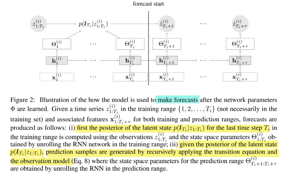
represent forecast distribution, in terms of \(K\) Monte Carlo samples

• \(\hat{z}_{k, T_{i}+1: T_{i}+\tau}^{(i)} \sim p\left(z_{T_{i}+1: T_{i}+\tau}^{(i)} \mid z_{1: T_{i}}^{(i)}, \mathbf{x}_{1: T_{i}+\tau}^{(i)}, \Theta_{1: T_{i}+\tau}^{(i)}\right), \quad k=1, \ldots, K\).

Step 1) compute the posterior \(p\left(\boldsymbol{l}_{T_{i}}^{(i)} \mid z_{1: T_{i}}^{(i)}\right)\) for each time series \(z_{1: T_{i}}^{(i)}\)

• by unrolling RNN in the training range to obtain \(\Theta_{1: T_{i}}^{(i)}\)

• then use Kalman filtering algorithm

Step 2) unroll the RNN for the prediction range

• obtain \(\Theta_{T_{i}+1: T_{i}+\tau}^{(i)}\)

Step 3) generate prediction samples

• by recursively applying above equations \(K\) times