(paper) FEDformer ; Frequency Enhanced Decomposed Transformer for Long-term TS Forecasting

FEDformer : Frequency Enhanced Decomposed Transformer for Long-term TS Forecasting (2022)

Contents

1. Abstract
2. Introduction
3. Compact Representation of TS in Frequency Domain
4. Model Stucture
   1. FEDformer Framework
   2. Fourier Enhanced Structure
   3. Wavelet Enhanced Structure
   4. Mixture of Experts for ST decomposition
   5. Complexity Analysis

0. Abstract

Cons of Transformer

• (1) computationally expensive
• (2) unable to capture GLOBAL view

Proposal :

• TRANSFORMER with seasonal-trend DECOMPOSITION
  • Decomposition method :
    • captures global profile of TS
  • Transformer :
    • captures more detailed structure
• for LONG-term prediction …
  • most TS tend to have a sparse representation in well-known basis, such as Fourier Transform

\(\rightarrow\) propose FEDformer

1. Introduction

LONG-term TS forecasting

• RNN :
  • cons : problem of gradient vanishing/exploding
• Transformer :
  • pros : able to capture long-term dependencies
  • cons : tend to fail in capturing the OVERALL(=GLOBAL) characteristics of TS

Prediction for each timestep is made individually & independentlly

• likely to fail to capture the global property/statistics of TS as a whole
• to solve this…propose FEDformer
  • IDEA 1) incorporate S-T decomposition
  • IDEA 2) combine Fourier Analysis with Transformer

Key quetsion :

• which subset of frequency components should be used by Fourier Analysis?

• (common wisdom)

  • keep LOW frequency component
  • throw away HIGH frequency component

  \(\rightarrow\) NOT APPROPRIATE!

• solve this, by effectively exploiting the fact that

  TS tend to have SPARSE representations on a basis, like Fourier basis

  \(\rightarrow\) randomly select frequency components!

Contribution

1. propose FEDformer

2. propose Fourier enhanced blocks & Wavelet enhanced blocks

3. by randomly selecting a fixed number of Fourier components,

   achieve linear computational complexity & memory cost

2. Compact Reprsentation of TS in Frequency domain

TS : can be modeled in

• (1) TIME domain
• (2) FREQUENCY domain

\(\rightarrow\) this algorithm : frequency-domain operation with NN

keep compact representation of TS,

using a small number of selected Foureir components ( more efficient! )

Notation

(before Fourier Transform)

• \(m\) time series : \(X_{1}(t), \ldots, X_{m}(t)\)

(after Fourier Transform)

• \(X_{i}(t)\) becomes \(a_{i}=\left(a_{i, 1}, \ldots, a_{i, d}\right)^{\top} \in \mathbb{R}^{d}\)

• \(A=\left(a_{1}, a_{2}, \ldots, a_{m}\right)^{\top} \in \mathbb{R}^{m \times d}\).

  • row : each TS ( \(m\) )
  • col : each Fourier Component ( \(d\) )

  need to select a subset of Fourier components

  • select \(s\) out of \(d\) ( Uniformly at random )
  • randomly selected components :
    • \(i_{1}<i_{2}< ... < i_{s}\).

Selected components :

• \(i_{1}<i_{2}< ... < i_{s}\).
• matrix \(S \in\{0,1\}^{s \times d}\)
  • \(S_{i, k}=1\) if \(i=i_{k}\) and \(S_{i, k}=0\) otherwise.

Representation of MTS :

• \(A^{\prime}=A S^{\top} \in \mathbb{R}^{m \times s}\).

3. Model Structure

introduce 3 parts

• (1) overall structure of FEDformer
• (2) 2 subversion strutures for signal process
  • (2-1) Fourier basis
  • (2-2) Wavlet basis
• (3) mixture of experts mechanism for ST decomposition

3-1. FEDformer Framework

Notation

• input length = \(I\)
• output length = \(O\)
• hidden state of TS = \(D\)
• Input
  • of Encoder : \(I \times D\) matrix
  • of Decoder : \((I/2 + O) \times D\) matrix

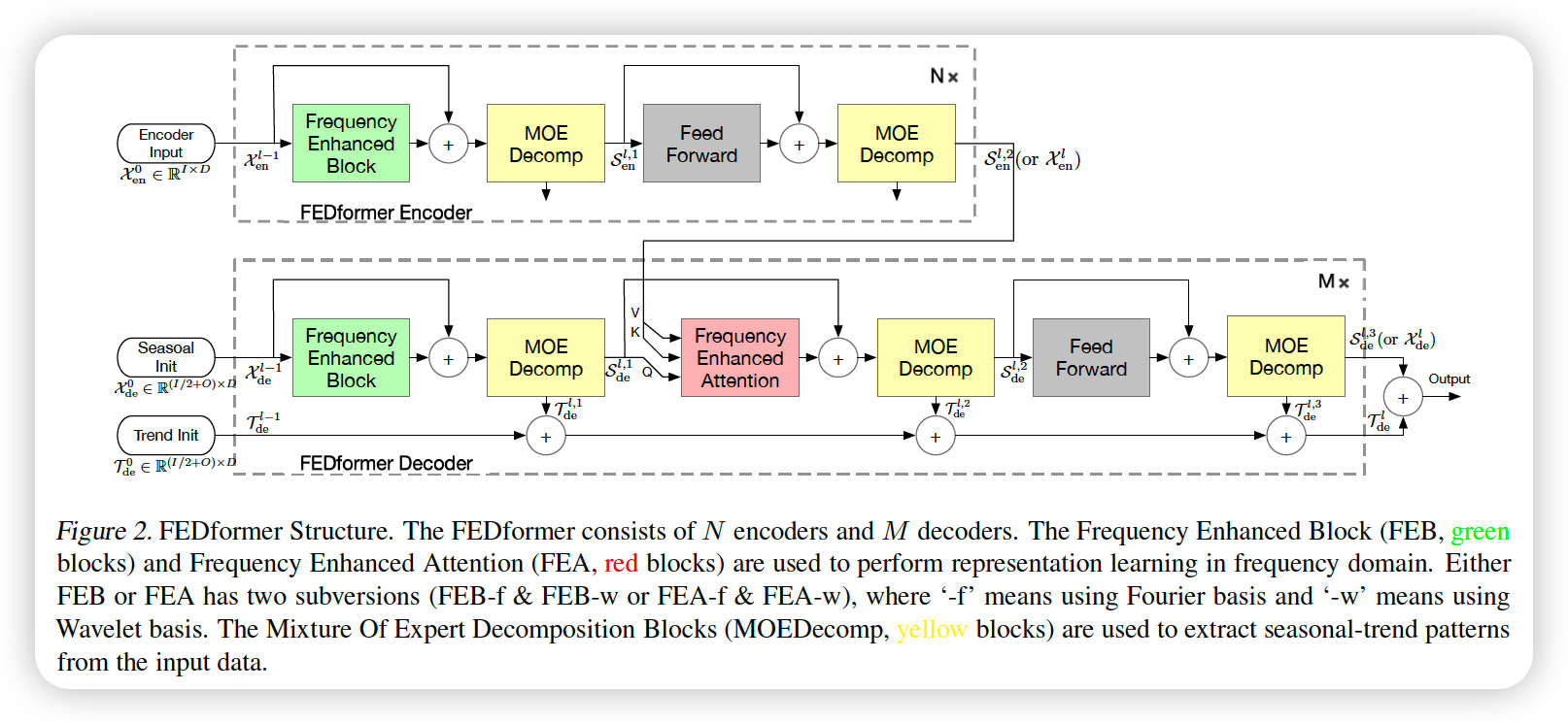
FEDformer Structure

• renovate Transformer as a deep decomposition architecture
• includes..
  • (1) FED ( Frequency Enhanced Block )
  • (2) FEA ( Frequency Enhanced Attention )
  • (3) MOEDcomp ( Mixture Of Experts Decomposition block )

a) Encoder

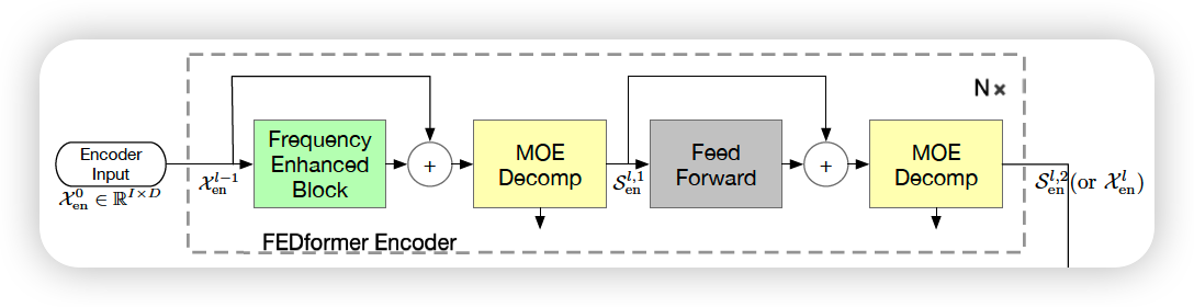
Encoder : multi-layer structure

( layer index : \(l \in\{1, \cdots, N\}\) )

• \(\mathcal{X}_{\mathrm{en}}^{0} \in \mathbb{R}^{I \times D}\) : embedded historical TS

• \(\mathcal{X}_{\mathrm{en}}^{l}=\operatorname{Encoder}\left(\mathcal{X}_{\text {en }}^{l-1}\right)\).

Encoder details :

\(\begin{aligned} \mathcal{S}_{\mathrm{en},-}^{l, 1} &=\operatorname{MOEDecomp}\left(\operatorname{FEB}\left(\mathcal{X}_{\mathrm{en}}^{l-1}\right)+\mathcal{X}_{\mathrm{en}}^{l-1}\right) \\ \mathcal{S}_{\mathrm{en}}^{l, 2}, &=\operatorname{MOEDecomp}\left(\text { FeedForward }\left(\mathcal{S}_{\mathrm{en}}^{l, 1}\right)+\mathcal{S}_{\mathrm{en}}^{l, 1}\right) \\ \mathcal{X}_{\mathrm{en}}^{l} &=\mathcal{S}_{\mathrm{en}}^{l, 2} \end{aligned}\).

• \(\mathcal{S}_{\mathrm{en}}^{l, i}, i \in\{1,2\}\) : seasonal component after the \(i\)-th decomposition block in the \(l\)-th layer

b) Decoder

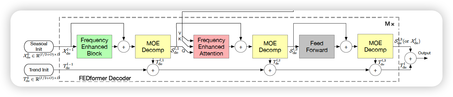
Decoder : multi-layer structure

( layer index : \(l \in\{1, \cdots, M\}\) )

• \(\mathcal{X}_{\mathrm{de}}^{l}, \mathcal{T}_{\mathrm{de}}^{l}=\operatorname{Decoder}\left(\mathcal{X}_{\mathrm{de}}^{l-1}, \mathcal{T}_{\mathrm{de}}^{l-1}\right)\).

Decoder details :

\(\begin{aligned} \mathcal{S}_{\mathrm{de}}^{l, 1}, \mathcal{T}_{\mathrm{de}}^{l, 1} &=\operatorname{MOEDecomp}\left(\mathrm{FEB}\left(\mathcal{X}_{\mathrm{de}}^{l-1}\right)+\mathcal{X}_{\mathrm{de}}^{l-1}\right) \\ \mathcal{S}_{\mathrm{de}}^{l, 2}, \mathcal{T}_{\mathrm{de}}^{l, 2} &=\operatorname{MOEDecomp}\left(\operatorname{FEA}\left(\mathcal{S}_{\mathrm{de}}^{l, 1}, \mathcal{X}_{\mathrm{en}}^{N}\right)+\mathcal{S}_{\mathrm{de}}^{l, 1}\right) \\ \mathcal{S}_{\mathrm{de}}^{l, 3}, \mathcal{T}_{\mathrm{de}}^{l, 3} &=\operatorname{MOEDecomp}\left(\text { FeedForward }\left(\mathcal{S}_{\mathrm{de}}^{l, 2}\right)+\mathcal{S}_{\mathrm{de}}^{l, 2}\right) \\ \mathcal{X}_{\mathrm{de}}^{l} &=\mathcal{S}_{\mathrm{de}}^{l, 3} \\ \mathcal{T}_{\mathrm{de}}^{l} &=\mathcal{T}_{\mathrm{de}}^{l-1}+\mathcal{W}_{l, 1} \cdot \mathcal{T}_{\mathrm{de}}^{l, 1}+\mathcal{W}_{l, 2} \cdot \mathcal{T}_{\mathrm{de}}^{l, 2}+\mathcal{W}_{l, 3} \cdot \mathcal{T}_{\mathrm{de}}^{l, 3} \end{aligned}\).

• \(\mathcal{S}_{\mathrm{de}}^{l, i}, \mathcal{T}_{\mathrm{de}}^{l, i}, i \in\{1,2,3\}\) : represent the seasonal & trend component, after the \(i\)-th decomposition block in the \(l\)-th layer

c) Final prediction

• sum of 2 refined decomposed components : \(\mathcal{W}_{\mathcal{S}} \cdot \mathcal{X}_{\mathrm{de}}^{M}+\mathcal{T}_{\mathrm{de}}^{M}\)
  • \(\mathcal{W}_{\mathcal{S}}\) : project seasonal component \(\mathcal{X}_{\mathrm{de}}^{M}\) to the target dim

3-2. Fourier Enhanced Structure

a) DFT ( Discrete Fourier Transform )

Notation

• \(\mathcal{F}\) : Fourier Transform
• \(\mathcal{F}^{-1}\) : Inverse Fourier Transform
• sequence of real numbers \(x_{n}\) ( TIME domain )
  • where \(n=1,2 \ldots N\).

DFT : \(X_{l}=\sum_{n=0}^{N-1} x_{n} e^{-i \omega l n}\)

( where \(l=1,2 \ldots L\) )

• \(i\) : imaginary unit
• \(X_{l}\) : sequence of complex numbers in frequency domain

iDFT : \(x_{n}=\sum_{l=0}^{L-1} X_{l} e^{i \omega l n}\)

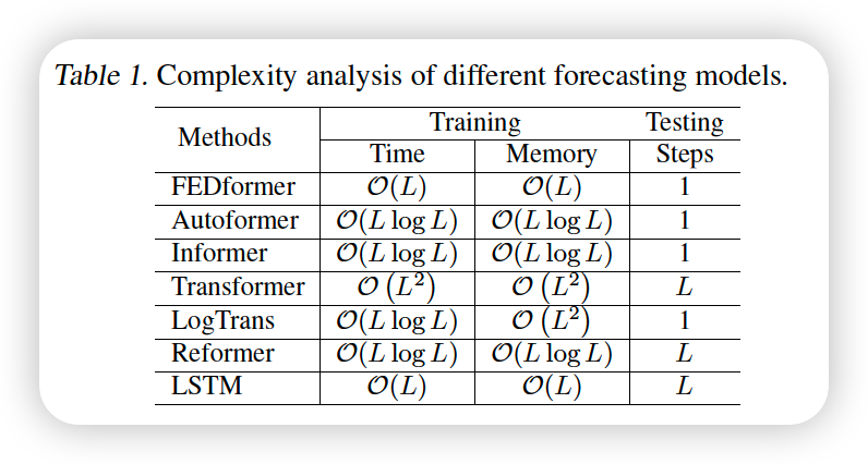
Complexity :

• DFT : \(O\left(N^{2}\right)\)

• FFT : \(O(N \log N)\)

• random subset of Fourier basis : \(O(N)\)

  ( + mode index before DFT and reverse DFT operations )

b) FEB-f ( Frequency Enhanced Block ( with Fourier Transform ) )

both used in Encoder & Decoder

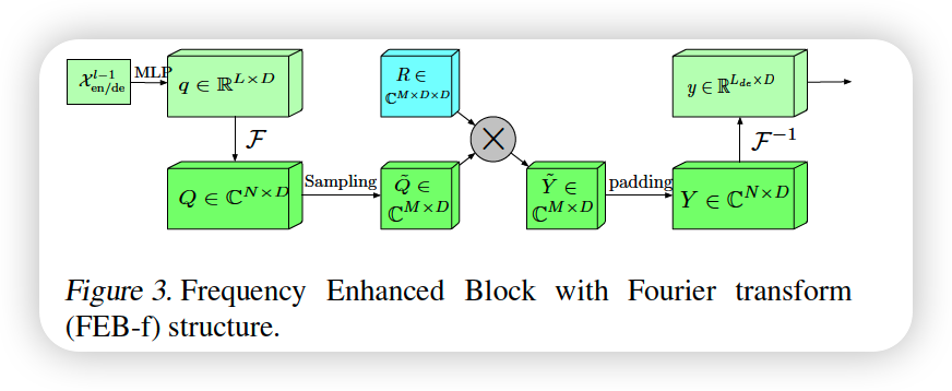
Process

• step 1) linear projected : \(\boldsymbol{q}=\boldsymbol{x} \cdot \boldsymbol{w}\)
  • where \(\boldsymbol{w} \in \mathbb{R}^{D \times D}\)
  • matrix notation : \(Q \in \mathbb{C}^{N \times D}\)
• step 2) convert TIME \(\rightarrow\) FREQUENCY domain : \(\boldsymbol{Q} = \mathcal{F}(\boldsymbol{q})\)
• step 3) select \(M\) Modes ( uniform randomly ) : \(\tilde{\boldsymbol{Q}}\)
• step 4) element-wise product with parameterized kernel : \(\boldsymbol{Y}=\boldsymbol{\tilde{Q}} \odot \boldsymbol{C}\)
• step 5) padding : \(\operatorname{Padding}(\tilde{\boldsymbol{Q}} \odot \boldsymbol{R})\)
• step 6) inverse transform : \(\mathrm{FEB}-\mathrm{f}(\boldsymbol{q})=\mathcal{F}^{-1}(\operatorname{Padding}(\tilde{\boldsymbol{Q}} \odot \boldsymbol{R}))\)
  • back to TIME domain

c) FEA-f ( Frequency Enhanced Attention ( with Fourier Transform ) )

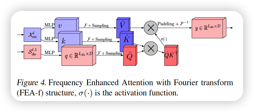
Expression of the canonical transformer

• \(\boldsymbol{q} \in \mathbb{R}^{L \times D}, \boldsymbol{k} \in \mathbb{R}^{L \times D}, \boldsymbol{v} \in \mathbb{R}^{L \times D}\).

Cross-attention

• Q come from decoder : \(\boldsymbol{q}=\boldsymbol{x}_{e n} \cdot \boldsymbol{w}_{q}\)
  • where \(\boldsymbol{w}_{q} \in \mathbb{R}^{D \times D}\)
• K & V from encoder : \(\boldsymbol{k}=\boldsymbol{x}_{d e} \cdot \boldsymbol{w}_{k}\) and \(\boldsymbol{v}=\boldsymbol{x}_{d e} \cdot \boldsymbol{w}_{v}\)
  • where \(\boldsymbol{w}_{k}, \boldsymbol{w}_{v} \in \mathbb{R}^{D \times D}\)
• attention :
  • \(\operatorname{Atten}(\boldsymbol{q}, \boldsymbol{k}, \boldsymbol{v})=\operatorname{Softmax}\left(\frac{\boldsymbol{q} \boldsymbol{k}^{\top}}{\sqrt{d_{q}}}\right) \boldsymbol{v}\).

in FEA-f, convert Q,K,V with FOURIER TRANSFORM

( with selected \(M\) modes )

• selected version after Fourier Transform :
  • \[\tilde{\boldsymbol{Q}} \in \mathbb{C}^{M \times D}, \boldsymbol{K} \in \mathbb{C}^{M \times D}, \tilde{\boldsymbol{V}} \in \mathbb{C}^{M \times D}\]
• FEA-f :
  • \(\tilde{\boldsymbol{Q}} =\operatorname{Select}(\mathcal{F}(\boldsymbol{q}))\).
  • \(\tilde{\boldsymbol{K}}=\operatorname{Select}(\mathcal{F}(\boldsymbol{k}))\).
  • \(\tilde{\boldsymbol{V}}=\operatorname{Select}(\mathcal{F}(\boldsymbol{v}))\).
• \(\mathrm{FEA}-\mathrm{f}(\boldsymbol{q}, \boldsymbol{k}, \boldsymbol{v})=\mathcal{F}^{-1}\left(\operatorname{Padding}\left(\sigma\left(\tilde{\boldsymbol{Q}} \cdot \tilde{\boldsymbol{K}}^{\top}\right) \cdot \tilde{\boldsymbol{V}}\right)\right)\).
  • use softmax/tanh for activation function

3-3. Wavelet Enhanced Structure

a) DWT ( Discrete Wavelet Transform )

b) FEB-w ( Frequency Enhanced Block ( with Wavelet Transform ) )

c) FEA-w ( Frequency Enhanced Attention ( with Wavelet Transform ) )

3-4. Mixture of Experts for ST decomposition

extracting trend can be hard with FIXED window average pooling

\(\rightarrow\) use MOEDecomp ( Mixture of Experts Decomposition block )

contains a set of average filters with different sizes,

to extract multiple trend components from the input signal

\(\mathbf{X}_{\text {trend }}=\operatorname{Softmax}(L(x)) *(F(x))\).

• \(F(\cdot)\) : set of average pooling filters
• \(\operatorname{Softmax}(L(x))\) : weights for mixing these extracted trends

3-5. Complexity Analysis