Univariate 2. 일반 선형확률 과정 ( General Linear Process ) (1)

“시계열 데이터 = 가우시안 백색잡음의 현재값과 과거값의 선형조합”*

\(Y_t = \epsilon_t + \psi_1\epsilon_{t-1} + \psi_2\epsilon_{t-2} + \cdots\).

where \(\epsilon_i \sim i.i.d.~WN(0, \sigma_{\epsilon_i}^2)~and~\displaystyle \sum_{i=1}^{\infty}\psi_i^2 < \infty\).

세부 알고리즘:

WN(White Noise)
MA(Moving Average)
AR(Auto-Regressive)
ARMA(Auto-Regressive Moving Average)
ARMAX(ARMA with eXogenous variables)

1. WN (White Noise)

(1) White Noise (백색 잡음)의 2가지 특징

[1] 잔차 (Residual)는 정규분포를 따른다

1) 정규 분포
- \(\begin{align*} \{\epsilon_t : t = \dots, -2, -1, 0, 1, 2, \dots\} \sim N(0,\sigma^2_{\epsilon_t}) \\ \end{align*}\).
  
  where \(\epsilon_t \sim i.i.d\)
2) mean=0, var=constant
- \(\epsilon_t = Y_t - \hat{Y_t}\).
  - \(E(\epsilon_t) = 0\).
  - \(Var(\epsilon_t) = \sigma^2_{\epsilon_t}\).

[2] 잔차들이 시간의 흐름에 따라 “상관성이 없어야” 한다

ACF (자기 상관 함수)를 통해 Autocorrelation=0인지 확인해야!
공분산 (Covariance)
- \(Cov(Y_s, Y_k)\) = \(E[(Y_s-E(Y_s))\)\((Y_k-E(Y_k))]\) = \(\gamma_{s,k}\)
자기상관함수 (Autocorrelation Function)
- \(Corr(Y_s, Y_k)\) = \(\dfrac{Cov(Y_s, Y_k)}{\sqrt{Var(Y_s)Var(Y_k)}}\) = \(\dfrac{\gamma_{s,k}}{\sqrt{\gamma_s \gamma_k}}\).
편자기상관함수 (Partial Autocorrelation Function)
- \(Corr[(Y_s-\hat{Y}_s, Y_{s-t}-\hat{Y}_{s-t})]\) for \(1<t<k\).

(2) Summary

강정상 과정(Stictly Stationary Process)
[공분산]
- lag(시차)=0 이면 \(\rightarrow\) 공분산 = 확률 분포의 분산
- lag(시차)\(\neq\)0 이면 \(\rightarrow\) 공분산 = 0
- \(\gamma_i = \begin{cases} \text{Var}(\epsilon_t) & \;\; \text{ for } i = 0 \\ 0 & \;\; \text{ for } i \neq 0 \end{cases}\).
[자기상관계수]
- lag(시차)=0 이면 \(\rightarrow\) 자기상관계수 = 1
- lag(시차)\(\neq\)0 이면 \(\rightarrow\) 자기상관계수 = 0
- \(\rho_i = \begin{cases} 1 & \;\; \text{ for } i = 0 \\ 0 & \;\; \text{ for } i \neq 0 \end{cases}\).

(3) Example

from scipy import stats
import matplotlib.pyplot as plt
import numpy as np

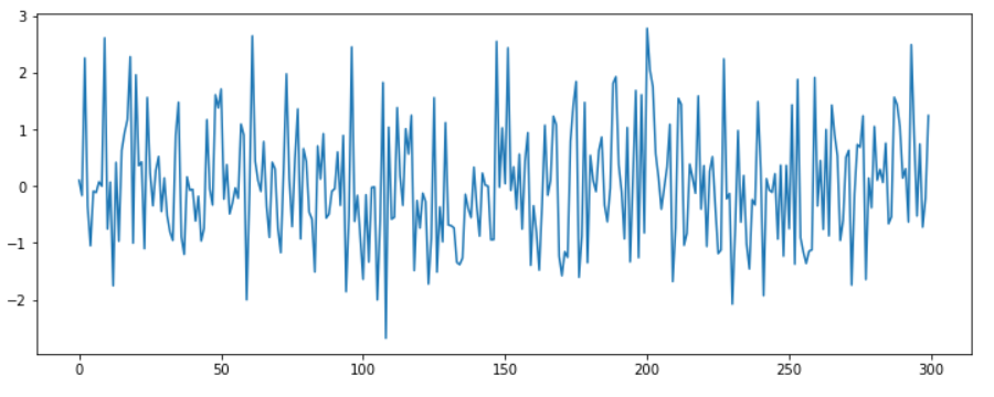
a) Gaussian WN

plt.plot(stats.norm.rvs(size=300))

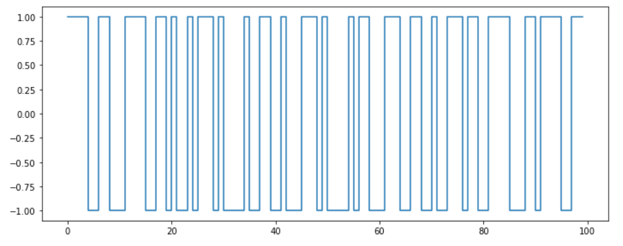
b) Bernoulli WN

( 반드시 Gaussian일 필요는 X )

samples = stats.bernoulli.rvs(0.5, size=100) * 2 - 1
plt.step(np.arange(len(samples)), samples)
plt.ylim(-1.1, 1.1)

2. MA (Moving Average)

(1) MA(\(q\))

알고리즘의 차수(\(q\))가 유한한 Gaussian WN의 Linear Combination

\(Y_t = \epsilon_t + \theta_1\epsilon_{t-1} + \theta_2\epsilon_{t-2} + \cdots + \theta_q\epsilon_{t-q}\).

where \(\epsilon_i \sim i.i.d.~WN(0, \sigma_{\epsilon_i}^2)~and~\displaystyle \sum_{i=1}^{\infty}\theta_i^2 < \infty\)

위 식을 정리하자면…

\[\begin{align*} Y_t &= \epsilon_t + \theta_1\epsilon_{t-1} + \theta_2\epsilon_{t-2} + \cdots + \theta_q\epsilon_{t-q} \\ &= \epsilon_t + \theta_1L\epsilon_t + \theta_2L^2\epsilon_t + \cdots + \theta_qL^q\epsilon_t \\ &= (1 + \theta_1L + \theta_2L^2 + \cdots + \theta_qL^q)\epsilon_t \\ &= \theta(L)\epsilon_t \\ \end{align*}\]

where \(\epsilon_{t-1} = L\epsilon_t~and~\epsilon_{t-2} = L^2\epsilon_t\)

(2) MA(1)

\(Y_t = \epsilon_t + \theta_1\epsilon_{t-1}\).

( Mean & Variance )

\(E(Y_t) = 0\).
\(Var(Y_t)=\sigma_{\epsilon_i}^2 + \theta_1^2\sigma_{\epsilon_i}^2\).

( Covariance )

\(Cov(Y_t, Y_{t-1})= \theta_1 \sigma_{\epsilon_{i}}^2\).
\(Cov(Y_t, Y_{t-2})= 0\).

( Correlation )

\(Corr(Y_t, Y_{t-1}) = \rho_1 = \dfrac{\theta_1}{1+\theta_1^2}\).
\(Corr(Y_t, Y_{t-i}) = \rho_i = 0~~for~~i > 1\).

[ Proof ]

\(E(Y_t) = E(\epsilon_t + \theta_1\epsilon_{t-1}) = E(\epsilon_t) + \theta_1E(\epsilon_{t-1}) = 0\).
\(\begin{aligned} Var(Y_t) &= E[(\epsilon_t + \theta_1\epsilon_{t-1})^2]-0^2 \\ &= E(\epsilon_t^2) + 2\theta_1E(\epsilon_{t}\epsilon_{t-1}) + \theta_1^2E(\epsilon_{t-1}^2) \\ &= (\sigma_{\epsilon_i}^2 +0^2)+ 2 \theta_1 \cdot 0 + \theta_1^2 (\sigma_{\epsilon_i}^2 +0^2) \\ &= \sigma_{\epsilon_i}^2 + \theta_1^2\sigma_{\epsilon_i}^2 \end{aligned}\).
\(\begin{aligned}Cov(Y_t, Y_{t-1}) &= \gamma_1 \\&= \text{E} \left[ (\epsilon_t + \theta_1 \epsilon_{t-1})(\epsilon_{t-1} + \theta_1 \epsilon_{t-2}) \right] \\ &= E (\epsilon_t \epsilon_{t-1}) + \theta_1 E (\epsilon_t \epsilon_{t-2}) + \theta_1 E (\epsilon_{t-1}^2) + \theta_1^2 E (\epsilon_{t-1} \epsilon_{t-2}) \\ &= 0 + \theta_1 \cdot 0 + \theta_1 (\sigma_{\epsilon_{i}}^2+0^2) + \theta_1^2 \cdot 0 \\ &= \theta_1 \sigma_{\epsilon_{i}}^2\end{aligned}\).
\(\begin{aligned}Cov(Y_t, Y_{t-2}) &= \gamma_2 \\&= \text{E} \left[ (\epsilon_t + \theta_1 \epsilon_{t-1})(\epsilon_{t-2} + \theta_1 \epsilon_{t-3}) \right] \\ &= E (\epsilon_t \epsilon_{t-2}) + \theta_1 E (\epsilon_t \epsilon_{t-3}) + \theta_1 E (\epsilon_{t-1} \epsilon_{t-2}) + \theta_1^2 E (\epsilon_{t-1} \epsilon_{t-3}) \\ &= 0 + \theta_1 \cdot 0 + \theta_1 \cdot 0 + \theta_1^2 \cdot 0 \\ &= 0 \end{aligned}\).

(3) MA(2)

\(Y_t = \epsilon_t + \theta_1\epsilon_{t-1} + \theta_2\epsilon_{t-2}\).

( Mean & Variance )

\(E(Y_t) =0\).
\(Var(Y_t) = \sigma_{\epsilon_i}^2 + \theta_1^2\sigma_{\epsilon_i}^2 + \theta_2^2\sigma_{\epsilon_i}^2\).

( Covariance )

\(Cov(Y_t, Y_{t-1}) = (\theta_1 + \theta_1\theta_2) \sigma_{\epsilon_{i}}^2\).
\(Cov(Y_t, Y_{t-2}) =\theta_2 \sigma_{\epsilon_{i}}^2\).
\(Cov(Y_t, Y_{t-i}) = \gamma_i = 0~~for~~i > 2\).

( Correlation )

\(Corr(Y_t, Y_{t-1}) = \rho_1 = \dfrac{\theta_1 + \theta_1 \theta_2}{1+\theta_1^2+\theta_2^2}\).
\(Corr(Y_t, Y_{t-2}) = \rho_2 = \dfrac{\theta_2}{1+\theta_1^2+\theta_2^2}\).
\[Corr(Y_t, Y_{t-i}) = \rho_i = 0~~for~~i > 2\]

[ Proof ]

\(E(Y_t) = E(\epsilon_t + \theta_1\epsilon_{t-1} + \theta_2\epsilon_{t-2}) = E(\epsilon_t) + \theta_1E(\epsilon_{t-1}) + \theta_2E(\epsilon_{t-2}) = 0\).
\(\begin{aligned} Var(Y_t) &= E[(\epsilon_t + \theta_1\epsilon_{t-1} + \theta_2\epsilon_{t-2})^2] \\ &= (\sigma_{\epsilon_i}^2+0^2) + \theta_1^2(\sigma_{\epsilon_i}^2+0^2) + \theta_2^2(\sigma_{\epsilon_i}^2+0^2) \end{aligned}\).
\(.\begin{aligned}Cov(Y_t, Y_{t-1}) &= \gamma_1 \\&= \text{E} \left[ (\epsilon_t + \theta_1 \epsilon_{t-1} + \theta_2\epsilon_{t-2})(\epsilon_{t-1} + \theta_1 \epsilon_{t-2} + \theta_2\epsilon_{t-3}) \right] \\ &= (\theta_1 + \theta_1\theta_2) \sigma_{\epsilon_{i}}^2 \end{aligned}\).
\(\begin{aligned} Cov(Y_t, Y_{t-2}) &= \gamma_2 \\&= \text{E} \left[ (\epsilon_t + \theta_1 \epsilon_{t-1} + \theta_2\epsilon_{t-2})(\epsilon_{t-2} + \theta_1 \epsilon_{t-3} + \theta_2\epsilon_{t-4}) \right] \\ &= \theta_2 \sigma_{\epsilon_{i}}^2 \end{aligned}\).
\(Cov(Y_t, Y_{t-i}) = \gamma_i = 0~~for~~i > 2\).

(4) MA(q)

\(\begin{aligned} Corr(Y_t, Y_{t-i}) = \rho_i &= \begin{cases} \dfrac{\theta_i + \theta_1\theta_{i-1} + \theta_2\theta_{i-2} + \cdots + \theta_q\theta_{i-q}}{1 + \theta_1^2 + \cdots + \theta_q^2} & \text{ for } i= 1, 2, \cdots, q \\ 0 & \text{ for } i > q \\ \end{cases} \end{aligned}\).

Stationarity Condition of MA(1): \(\mid \theta_1\mid < 1\)
Stationarity Condition of MA(2): \(\mid \theta_2\mid < 1\), \(\theta_1 + \theta_2 > -1\), \(\theta_1 - \theta_2 < 1\)

(5) Example

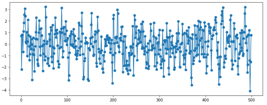
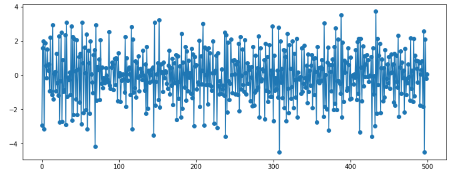
MA(1)

ar_params = np.array([])
ma_params = np.array([0.9])
ar, ma = np.r_[1, -ar_params], np.r_[1, ma_params]

print(ar)
print(ma)
#------------------------#
[1.]
[1.  0.9]

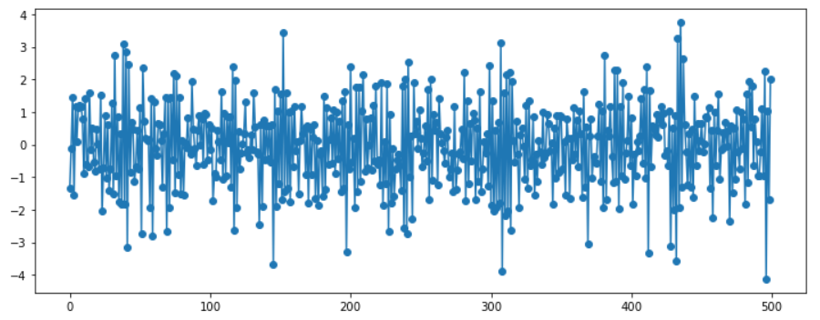
y = sm.tsa.ArmaProcess(ar, ma).generate_sample(500, burnin=50)
plt.plot(y, 'o-')

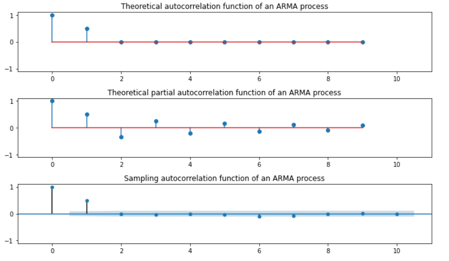
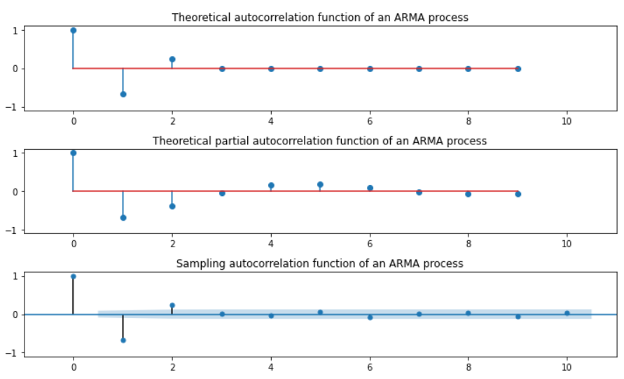
plt.stem().acf : auto correlation function
plt.stem().pacf : partial auto correlation function
sm.graphics.tsa.plot_acf : auto correlation function with SAMPLING

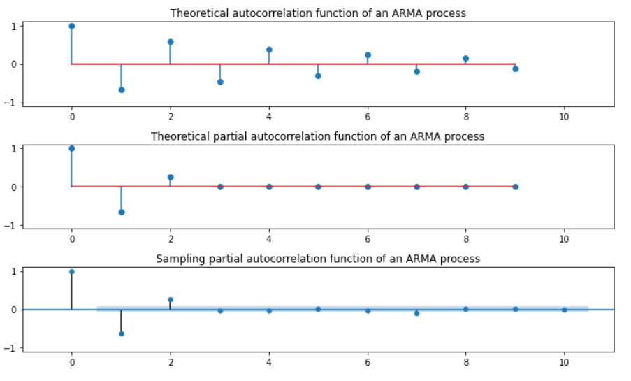
plt.figure(figsize=(10, 6))
plt.subplot(311)
plt.stem(sm.tsa.ArmaProcess(ar, ma).acf(lags=10))
plt.xlim(-1, 11)
plt.ylim(-1.1, 1.1)
plt.title("Theoretical autocorrelation function of an ARMA process")
#----------------------------------------------------------------------#
plt.subplot(312)
plt.stem(sm.tsa.ArmaProcess(ar, ma).pacf(lags=10))
plt.xlim(-1, 11)
plt.ylim(-1.1, 1.1)
plt.title("Theoretical partial autocorrelation function of an ARMA process")
#----------------------------------------------------------------------#
sm.graphics.tsa.plot_acf(y, lags=10, ax=plt.subplot(313))
plt.xlim(-1, 11)
plt.ylim(-1.1, 1.1)
plt.title("Sampling autocorrelation function of an ARMA process")
plt.tight_layout()
plt.show()

MA(2)

ar_params = np.array([])
ma_params = np.array([-1, 0.6])
ar, ma = np.r_[1, -ar_params], np.r_[1, ma_params]

print(ar)
print(ma)
#------------------------
[1.]
[ 1.  -1.   0.6]

y = sm.tsa.ArmaProcess(ar, ma).generate_sample(500, burnin=50)
plt.plot(y, 'o-')

plt.figure(figsize=(10, 6))
plt.subplot(311)
plt.stem(sm.tsa.ArmaProcess(ar, ma).acf(lags=10))
plt.xlim(-1, 11)
plt.ylim(-1.1, 1.1)
plt.title("Theoretical autocorrelation function of an ARMA process")
#----------------------------------------------------------------------#
plt.subplot(312)
plt.stem(sm.tsa.ArmaProcess(ar, ma).pacf(lags=10))
plt.xlim(-1, 11)
plt.ylim(-1.1, 1.1)
plt.title("Theoretical partial autocorrelation function of an ARMA process")
#----------------------------------------------------------------------#
sm.graphics.tsa.plot_acf(y, lags=10, ax=plt.subplot(313))
plt.xlim(-1, 11)
plt.ylim(-1.1, 1.1)
plt.title("Sampling autocorrelation function of an ARMA process")
plt.tight_layout()
plt.show()

3. AR (Auto-Regressive)

\(AR(p)\): 알고리즘의 차수(\(p\))가 유한한 자기자신의 과거값들의 Linear Combination

( 시차(Lag)가 증가해도 , ACF가 0이 되지 않는 경우, MA 모형을 사용할 경우 차수는 \(\infty\) 여야 하는 문제 상황! )

\(Y_t = \phi_1Y_{t-1} + \phi_2Y_{t-2} + \cdots + \phi_pY_{t-p} + \epsilon_t\).

where \(\epsilon_i \sim i.i.d.~WN(0, \sigma_{\epsilon_i}^2)~and~\displaystyle \sum_{i=1}^{\infty}\phi_i^2 < \infty\)

위 식을 정리하면…

\(Y_t - \phi_1Y_{t-1} - \phi_2Y_{t-2} - \cdots - \phi_pY_{t-p} = \epsilon_t\).
\(Y_t - \phi_1LY_t - \phi_2L^2Y_t - \cdots - \phi_pL^pY_t= \epsilon_t\).
\((1 - \phi_1L - \phi_2L^2 - \cdots - \phi_pL^p)Y_t = \epsilon_t\).
\(\phi(L)Y_t = \epsilon_t\).

(1) AR(1)

\(Y_t = \phi_1 Y_{t-1} + \epsilon_t = MA(\infty)\).

( Mean & Variance )

\(E(Y_t) = \mu = 0~~if~~\phi_1 \neq 1\).
\(Var(Y_t) =\gamma_0= \dfrac{\sigma_{\epsilon_i}^2}{1-\phi_1^2}~~if~~\phi_1^2 \neq 1\).

( Covariance )

\(Cov(Y_t, Y_{t-1})=\gamma_1 = \dfrac{\phi_1 \sigma_{\epsilon_{i}}^2}{1 - \phi_1^2}\).
\(Cov(Y_t, Y_{t-2}) = \gamma_2 = \dfrac{\phi_1^2 \sigma_{\epsilon_{i}}^2}{1 - \phi_1^2}\).

( Correlation )

\[Corr(Y_t, Y_{t-1}) = \rho_1 = \phi_1\]
\(Corr(Y_t, Y_{t-2}) = \rho_2 = \phi_1^2\).
\(Corr(Y_t, Y_{t-i}) = \rho_i = \phi_1^i\).

[ Proof는 생략 ]

Summary

\(\phi_1 = 0\) : White Noise
\(\phi_1 < 0\) : 부호를 바꿔가면서(진동하면서) 지수적으로 감소
\(\phi_1 > 0\) : 시차가 증가하면서 자기상관계수는 지수적으로 감소
\(\phi_1 = 1\): 비정상성인 Random Walk
- \(Y_t = Y_{t-1} + \epsilon_t\).
- \(Var(Y_t) > Var(Y_{t-1})\).
Stationarity Condition: \(\mid \phi_1\mid < 1\)

(2) AR(2)

\(Y_t = \phi_1 Y_{t-1} + \phi_2 Y_{t-2} + \epsilon_t = MA(\infty)\).

( Mean & Variance )

\(E(Y_t) = \mu = 0~~if~~\phi_1 + \phi_2 \neq 1\).

( Covariance(“Yule-Walker Equation”) )

\(Cov(Y_t, Y_{t-1})= \phi_1 \gamma_{i-1} + \phi_2 \gamma_{i-2}\).

( Correlation )

\(\begin{aligned}Corr(Y_t, Y_{t-i}) &= \rho_i \\&= \phi_1 \rho_{i-1} + \phi_2 \rho_{i-2}\end{aligned}\).
\(\begin{aligned} \rho_1 &= \dfrac{\phi_1}{1-\phi_2} \\ & \vdots \\ \rho_2 &= \dfrac{\phi_1^2 + \phi_2(1-\phi_2)}{1-\phi_2} \\ & \vdots \\ \rho_i &= \left( 1+\dfrac{1+\phi_2}{1-\phi_2} \cdot i \right)\left(\dfrac{\phi_1}{2} \right)^i \end{aligned}\).

[ Proof는 생략 ]

Summary

시차가 증가하면서 자기상관계수의 절대값은 지수적으로 감소
진동 주파수에 따라 다르지만 진동 가능
Stationarity Condition: \(\mid \phi_1\mid < 1\), \(\phi_1 + \phi_2 < 1\), \(\phi_2 - \phi_1 < 1\)

(3) Example

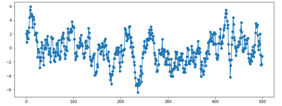
AR(1) .. \(\phi_1 = 0.9\)

ar_params = np.array([0.9])
ma_params = np.array([])
ar, ma = np.r_[1, -ar_params], np.r_[1, ma_params]
print(ar)
print(ma)
#------------------------------------------------
[ 1.  -0.9]
[1.]

y = sm.tsa.ArmaProcess(ar, ma).generate_sample(500, burnin=50)
plt.plot(y, 'o-')

plt.figure(figsize=(10, 6))
plt.subplot(311)
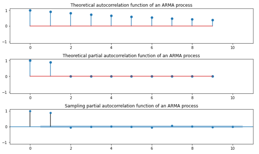
plt.stem(sm.tsa.ArmaProcess(ar, ma).acf(lags=10))
plt.xlim(-1, 11)
plt.ylim(-1.1, 1.1)
plt.title("Theoretical autocorrelation function of an ARMA process")
#------------------------------------------------------#
plt.subplot(312)
plt.stem(sm.tsa.ArmaProcess(ar, ma).pacf(lags=10))
plt.xlim(-1, 11)
plt.ylim(-1.1, 1.1)
plt.title("Theoretical partial autocorrelation function of an ARMA process")
#------------------------------------------------------#
sm.graphics.tsa.plot_pacf(y, lags=10, ax=plt.subplot(313))
plt.xlim(-1, 11)
plt.ylim(-1.1, 1.1)
plt.title("Sampling partial autocorrelation function of an ARMA process")
plt.tight_layout()
plt.show()

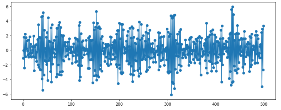
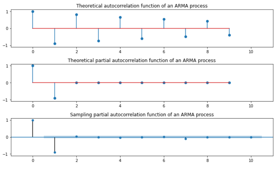
AR(1) .. \(\phi_1 = -0.9\)

ar_params = np.array([-0.9])
ma_params = np.array([])
ar, ma = np.r_[1, -ar_params], np.r_[1, ma_params]
print(ar)
print(ma)
#------------------------------------------------
[ 1.  0.9]
[1.]

( 이하 코드 동일 )

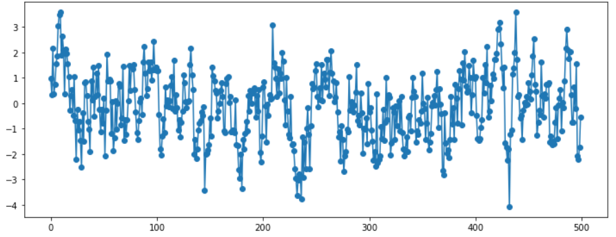
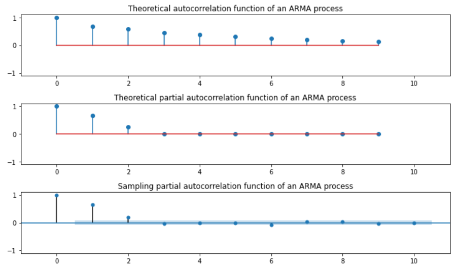
AR(2) … \(\phi_1 = 0.5, \phi_2=0.25\)

ar_params = np.array([0.5, 0.25])
ma_params = np.array([])
ar, ma = np.r_[1, -ar_params], np.r_[1, ma_params]
print(ar)
print(ma)
#------------------------------------------------
[ 1.  -0.5, -0.25]
[1.]

( 이하 코드 동일 )

AR(2) … \(\phi_1 = -0.5, \phi_2=0.25\)

ar_params = np.array([-0.5, 0.25])
ma_params = np.array([])
ar, ma = np.r_[1, -ar_params], np.r_[1, ma_params]
print(ar)
print(ma)
#------------------------------------------------
[ 1.  0.5, -0.25]
[1.]

( 이하 코드 동일 )

4. Relation of MA & AR

가역성 조건(Invertibility Condition):

1) \(MA(q)\) -> \(AR(\infty)\): 변환 후, AR 모형이 Stationary Condition을 만족하면 **“가역성(Invertibility)” **
2) \(AR(p)\) -> \(MA(\infty)\): 여러개 모형변환 가능!

( BUT, “Invertibility” 조건을 만족하는 MA 모형은 ONLY 1개 )

Twitter Facebook LinkedIn

Classical Time Series Algorithm 3

Seunghan Lee

Univariate 2. 일반 선형확률 과정 ( General Linear Process ) (1)

1. WN (White Noise)

(1) White Noise (백색 잡음)의 2가지 특징

(2) Summary

(3) Example

2. MA (Moving Average)

(1) MA(\(q\))

(2) MA(1)

(3) MA(2)

(4) MA(q)

(5) Example

MA(1)

MA(2)

3. AR (Auto-Regressive)

(1) AR(1)

Summary

(2) AR(2)

Summary

(3) Example

AR(1) .. \(\phi_1 = 0.9\)

AR(1) .. \(\phi_1 = -0.9\)

AR(2) … \(\phi_1 = 0.5, \phi_2=0.25\)

AR(2) … \(\phi_1 = -0.5, \phi_2=0.25\)

4. Relation of MA & AR

You May Also Enjoy