
Sequences, Time Series and Prediction
( 참고 : coursera의 Sequences, Time Series and Prediction 강의 )
[ Week 1 ] Sequence and Predictions
- Import Packages
- Plotting Function,
plot_series - TS with trend
- TS with seasonality
- TS with trend + seasonality
- TS with trend+seasonality+noise
- Preparing Forecast
- Forecast
1. Import Packages
import numpy as np
import matplotlib.pyplot as plt
import tensorflow as tf
from tensorflow import keras

print(tf.__version__)
2.6.0
2. Plotting Function, plot_series
def plot_series(time, series, format="-", start=0, end=None, label=None):
    plt.plot(time[start:end], series[start:end], format, label=label)
    plt.xlabel("Time")
    plt.ylabel("Value")
    if label:
        plt.legend(fontsize=14)
    plt.grid(True)
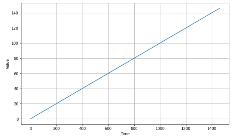
3. TS with trend
(1) trend
def trend(time, slope=0):
    return slope * time
(2) make synthetic dataset
time = np.arange(4 * 365 + 1)
series = trend(time, 0.1)
print(time)
print(series)
[   0    1    2 ... 1458 1459 1460]
[0.000e+00 1.000e-01 2.000e-01 ... 1.458e+02 1.459e+02 1.460e+02]
(3) plotting
plt.figure(figsize=(10, 6))
plot_series(time, series)
plt.show()
4. TS with seasonality
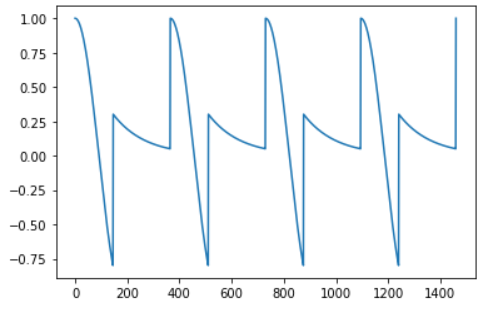
(1) seasonal_pattern
( 임의의 seasonal pattern을 만들어내는 함수 )
def seasonal_pattern(season_time):
    return np.where(season_time < 0.4,
                    np.cos(season_time * 2 * np.pi), # if TRUE
                    1 / np.exp(3 * season_time))     # if FALSE
example= (time % 365) / 365
plt.plot(example)
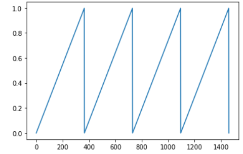
plt.plot(seasonal_pattern(example))
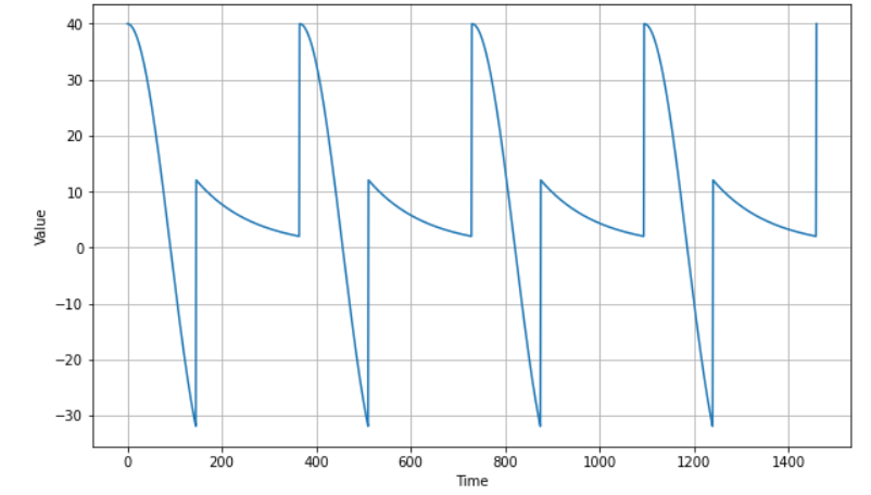
(2) seasonality
def seasonality(time, period, amplitude=1, phase=0):
    season_time = ((time + phase) % period) / period
    season_pattern = seasonal_pattern(season_time)
    return amplitude * season_pattern
진폭 ( scale )을 40배로!
365일마다 반복되는 seasonality
amplitude = 40
period=365
series = seasonality(time, period=period, amplitude=amplitude)
시각화
plt.figure(figsize=(10, 6))
plot_series(time, series)
plt.show()
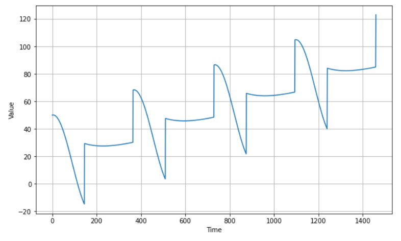
5. TS with trend + seasonality
slope = 0.05
baseline=10

series = baseline + trend(time, slope) + seasonality(time, period=period, amplitude=amplitude)
plt.figure(figsize=(10, 6))
plot_series(time, series)
plt.show()
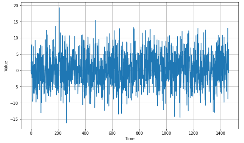
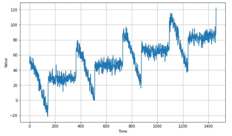
6. TS with trend+seasonality+noise
White Noise를 생성하는 함수
def white_noise(time, noise_level=1, seed=None):
    rnd = np.random.RandomState(seed)
    return rnd.randn(len(time)) * noise_level
Noise 수준 : \(5 \times N(0,1)\)
noise_level = 5
noise = white_noise(time, noise_level, seed=42)
plt.figure(figsize=(10, 6))
plot_series(time, noise)
plt.show()
위에서 생성한 time series에 noise를 더한 뒤 시각화
series += noise

plt.figure(figsize=(10, 6))
plot_series(time, series)
plt.show()
7. Preparing Forecast
(1) make synthetic dataset
hyperparameters
baseline = 10
amplitude = 40
slope = 0.05
noise_level = 5
trend + seasonality + noise
time = np.arange(4 * 365 + 1, dtype="float32")

series = baseline + trend(time, slope) + seasonality(time, period=365, amplitude=amplitude)

series += noise(time, noise_level, seed=42)
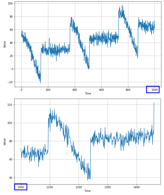
(2) Train & Validation Split
- ~1000개 : train
- 1001개~ : validation
split_time = 1000

time_train = time[:split_time]
x_train = series[:split_time]
time_valid = time[split_time:]
x_valid = series[split_time:]
Univariate Time Series
print(time_train.shape)
print(x_train.shape) # Univariate
print(time_valid.shape)
print(x_valid.shape) # Univariate
(1000,)
(1000,)
(461,)
(461,)
plt.figure(figsize=(10, 6))
plot_series(time_train, x_train)
plt.show()

plt.figure(figsize=(10, 6))
plot_series(time_valid, x_valid)
plt.show()
8. Forecast
(1) Naive Forecast
이전 시점의 값을 다음 시점의 예측값으로 사용
naive_forecast = series[split_time - 1:-1]
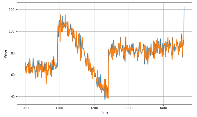
Validation 데이터의 예측 결과
- 전체 (time 1000~1461)
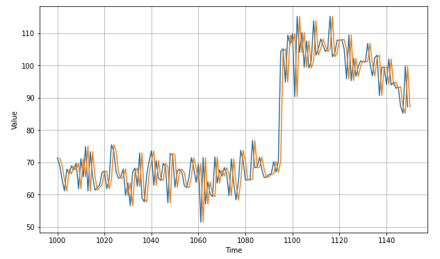
- 확대 (time 1000~1150)
# 전체
plt.figure(figsize=(10, 6))
plot_series(time_valid, x_valid)
plot_series(time_valid, naive_forecast)

# 확대
plt.figure(figsize=(10, 6))
plot_series(time_valid, x_valid, start=0, end=150)
plot_series(time_valid, naive_forecast, start=1, end=151)
예측 성능 (MSE & MAE)
print(keras.metrics.mean_squared_error(x_valid, naive_forecast).numpy())
print(keras.metrics.mean_absolute_error(x_valid, naive_forecast).numpy())
61.827534
5.937908
(2) Moving Average (MA)
window size를 지정해줘야
- “window size=1의 MA” = “naive forecast”
def moving_average_forecast(series, window_size):
  forecast = []
  for time in range(len(series) - window_size):
    forecast.append(series[time:time + window_size].mean())
  return np.array(forecast)
length 확인하기
series: 전체 데이터셋…train&valid ( = 0~1461 )moving_average_forecast(series, 30): 예측 결과…train&valid ( = 0~(1461-1430) )moving_avg: 예측 결과…valid ( = 1000 ~ 1461 )
moving_avg = moving_average_forecast(series, 30)[split_time - 30:]

print(len(series))
print(len(moving_average_forecast(series, 30)))
print(moving_avg)
1461
1431
461
예측 성능 (MSE & MAE)
print(keras.metrics.mean_squared_error(x_valid, moving_avg).numpy())
print(keras.metrics.mean_absolute_error(x_valid, moving_avg).numpy())
106.674576
7.142419
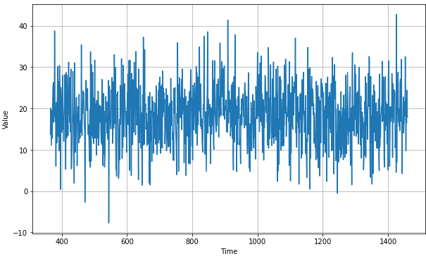
(3) 차분 후 MA
1년(=365일)전 값을 빼줌
- ex) 2021년 7월 29 값 - 2020년 7월 29일 값
lag=365
diff_series = (series[lag:] - series[:-lag])
diff_time = time[lag:]
1461일-365일 = 1096일
len(diff_series),len(diff_time)
(1096, 1096)
plt.figure(figsize=(10, 6))
plot_series(diff_time, diff_series)
plt.show()
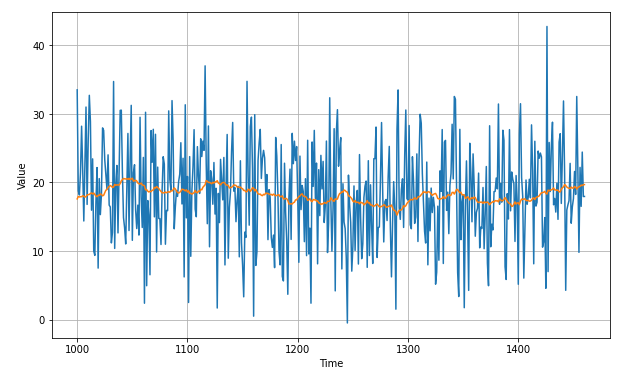
window_size=50
lag=365
diff_moving_avg = moving_average_forecast(diff_series, 50)[split_time - lag - window_size:]
plt.figure(figsize=(10, 6))
plot_series(time_valid, diff_series[split_time - lag:])
plot_series(time_valid, diff_moving_avg)
plt.show()
365일 전 값들을 다시 더해줘야!
diff_moving_avg_plus_past = series[split_time - lag:-lag] + diff_moving_avg

plt.figure(figsize=(10, 6))
plot_series(time_valid, x_valid)
plot_series(time_valid, diff_moving_avg_plus_past)
plt.show()
예측 성능 (MSE & MAE)
print(keras.metrics.mean_squared_error(x_valid, diff_moving_avg_plus_past).numpy())
print(keras.metrics.mean_absolute_error(x_valid, diff_moving_avg_plus_past).numpy())
52.973663
5.839311
(4) 차분 후 MA + smoothing
diff_moving_avg = moving_average_forecast(diff_series, 50)[split_time - lag - window_size:]
# BEFORE (smoothing X)
diff_moving_avg_plus_past = series[split_time - 365:-365] + diff_moving_avg

# AFTER (smoothing O)
diff_moving_avg_plus_smooth_past = moving_average_forecast(series[split_time - (lag+5):-(lag-5)], 10) + diff_moving_avg
plt.figure(figsize=(10, 6))
plot_series(time_valid, x_valid)
plot_series(time_valid, diff_moving_avg_plus_smooth_past)
plt.show()
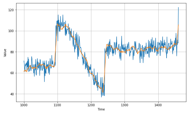
예측 성능 (MSE & MAE)
print(keras.metrics.mean_squared_error(x_valid, diff_moving_avg_plus_smooth_past).numpy())
print(keras.metrics.mean_absolute_error(x_valid, diff_moving_avg_plus_smooth_past).numpy())
33.452263
4.569442