
Sequences, Time Series and Prediction
( 참고 : coursera의 Sequences, Time Series and Prediction 강의 )
[ Week 2 ] DNN for Time Series
- Import Packages
- Dealing with
tf.data.Dataset - Single layer NN
- DNN
1. Import Packages
import tensorflow as tf
import numpy as np
import matplotlib.pyplot as plt
2. Dealing with tf.data.Dataset
tf.data.Dataset
dataset = tf.data.Dataset.range(10)
print(dataset)

for val in dataset:
   print(val.numpy())
<PrefetchDataset shapes: ((None, None), (None, None)), types: (tf.int64, tf.int64)>

0
1
2
3
4
5
6
7
8
9
dataset.window
size: window의 크기shift: window ~ window 의 shift 거리drop_remainder: True / False ( 아래에서 확인 )
dataset = tf.data.Dataset.range(10)
dataset1 = dataset.window(size=5, shift=1)
dataset2 = dataset.window(size=5, shift=1,drop_remainder=True)
for window_dataset in dataset1:
  for val in window_dataset:
    print(val.numpy(), end=" ")
  print()
#-----------------------------------#
for window_dataset in dataset2:
  for val in window_dataset:
    print(val.numpy(), end=" ")
  print()
0 1 2 3 4
1 2 3 4 5
2 3 4 5 6
3 4 5 6 7
4 5 6 7 8
5 6 7 8 9
6 7 8 9
7 8 9
8 9
9

0 1 2 3 4
1 2 3 4 5
2 3 4 5 6
3 4 5 6 7
4 5 6 7 8
5 6 7 8 9
dataset.flat_map(lambda x:f(x))
- list안에 담기도록 flatten 시키기
- batch size는 5로
dataset = tf.data.Dataset.range(10)
dataset = dataset.window(5, shift=1, drop_remainder=True)
dataset = dataset.flat_map(lambda window: window.batch(5))
for window in dataset:
  print(window.numpy())
[0 1 2 3 4]
[1 2 3 4 5]
[2 3 4 5 6]
[3 4 5 6 7]
[4 5 6 7 8]
[5 6 7 8 9]
dataset.map(lambda window: (window[:-1], window[-1:]))
- X,y부분으로 나누기
dataset = tf.data.Dataset.range(10)
dataset = dataset.window(5, shift=1, drop_remainder=True)
dataset = dataset.flat_map(lambda window: window.batch(5))
dataset = dataset.map(lambda window: (window[:-1], window[-1:]))
for x,y in dataset:
  print(x.numpy(), y.numpy())
[0 1 2 3] [4]
[1 2 3 4] [5]
[2 3 4 5] [6]
[3 4 5 6] [7]
[4 5 6 7] [8]
[5 6 7 8] [9]
dataset.shuffle(buffer_size=10)
- shuffle하기 ( buffer size = 데이터의 개수 )
dataset = tf.data.Dataset.range(10)
dataset = dataset.window(5, shift=1, drop_remainder=True)
dataset = dataset.flat_map(lambda window: window.batch(5))
dataset = dataset.map(lambda window: (window[:-1], window[-1:]))
dataset = dataset.shuffle(buffer_size=10)
for x,y in dataset:
  print(x.numpy(), y.numpy())
[2 3 4 5] [6]
[5 6 7 8] [9]
[0 1 2 3] [4]
[3 4 5 6] [7]
[1 2 3 4] [5]
[4 5 6 7] [8]
dataset.batch(2).prefetch(1)
- batch size = 2로 해서 불러오기
dataset = tf.data.Dataset.range(10)
dataset = dataset.window(5, shift=1, drop_remainder=True)
dataset = dataset.flat_map(lambda window: window.batch(5))
dataset = dataset.map(lambda window: (window[:-1], window[-1:]))
dataset = dataset.shuffle(buffer_size=10)
dataset = dataset.batch(2).prefetch(1)
for x,y in dataset:
  print("x = ", x.numpy())
  print("y = ", y.numpy())
3. Single layer NN
(1) dataset
split_time = 1000
time_train = time[:split_time]
x_train = series[:split_time]
time_valid = time[split_time:]
x_valid = series[split_time:]

window_size = 20
batch_size = 32
shuffle_buffer_size = 1000
print(x_train.shape)
print(x_valid.shape)
print(time_train.shape)
print(time_valid.shape)
(1000,)
(461,)
(1000,)
(461,)
위에서 봤던 data preprocessing을 사용한 windowed_dataset 함수
- dimension of X : 20 ( = window_size )
- dimension of Y : 1
하나의 배치의 shape : X = (32,20) & Y = (32,1)
def windowed_dataset(series, window_size, batch_size, shuffle_buffer):
  dataset = tf.data.Dataset.from_tensor_slices(series)
  dataset = dataset.window(window_size + 1, shift=1, drop_remainder=True)
  dataset = dataset.flat_map(lambda window: window.batch(window_size + 1))
  dataset = dataset.shuffle(shuffle_buffer).map(lambda window: (window[:-1], window[-1]))
  dataset = dataset.batch(batch_size).prefetch(1)
  return dataset
dataset = windowed_dataset(x_train, window_size, batch_size, shuffle_buffer_size)
(2) modeling
- step 1) layer들 만들기
- step 2)
tf.keras.models.Sequential()안에 layer 리스트 넣기 - step 3) compile
- loss function
- optimizer
- step 4) fitting
layer1 = tf.keras.layers.Dense(1,input_shape=[window_size])
model = tf.keras.models.Sequential([layer1])


model.compile(loss="mse", optimizer=tf.keras.optimizers.SGD(learning_rate=1e-6,
                                                            momentum=0.9))
model.fit(dataset,epochs=100,verbose=0)
layer1.get_weights()) 로 layer의 weight를 가져올 수 있음
(3) Prediction
forecast = []

for time in range(len(series) - window_size):
    y_hat = model.predict(series[time:time + window_size][np.newaxis])
	forecast.append(y_hat)
forecast의 길이 : 1461(X), 1441(O)
- 첫 예측은 t=1이 아니라, t=20+1=21부터 이루어짐
- 따라서, 21~1461까지 총 “1441”개의 예측값이 존재
len(forecast)
1441
validation 데이터 부분의 예측값에 대해서만 확인하기
- 1461-1000=461 개
forecast = forecast[split_time-window_size:]
len(forecast)
461
model의 prediction 결과의 dimension을 바꿔준다
results = np.array(forecast)[:, 0, 0]

print(forecast[0:5])
print(results[0:5])
[array([[68.06387]], dtype=float32),
 array([[69.79799]], dtype=float32),
 array([[71.91788]], dtype=float32),
 array([[69.33402]], dtype=float32),
 array([[65.159164]], dtype=float32)]

 array([68.06387 , 69.79799 , 71.91788 , 69.33402 , 65.159164],
      dtype=float32)
plt.figure(figsize=(10, 6))

plot_series(time_valid, x_valid)
plot_series(time_valid, results)
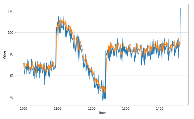
(4) Evaluation
tf.keras.metrics.mean_absolute_error(x_valid, results).numpy()
5.4876466
4. DNN
(1) 기본 구조
model = tf.keras.models.Sequential([
    tf.keras.layers.Dense(10, input_shape=[window_size], activation="relu"),
    tf.keras.layers.Dense(10, activation="relu"),
    tf.keras.layers.Dense(1)
])

model.compile(loss="mse", optimizer=tf.keras.optimizers.SGD(learning_rate=1e-6, momentum=0.9))
model.fit(dataset,epochs=100,verbose=0)
(2) Learning Rate Scheduler
model = tf.keras.models.Sequential([
    tf.keras.layers.Dense(10, input_shape=[window_size], activation="relu"),
    tf.keras.layers.Dense(10, activation="relu"),
    tf.keras.layers.Dense(1)
])

lr_schedule = tf.keras.callbacks.LearningRateScheduler(
    lambda epoch: 1e-8 * 10**(epoch / 20))
optimizer = tf.keras.optimizers.SGD(learning_rate=1e-8, momentum=0.9)
model.compile(loss="mse", optimizer=optimizer)
history = model.fit(dataset, epochs=100, callbacks=[lr_schedule], verbose=0)