(paper) A Time Series is Worth 64 Words ; Long-term Forecasting with Transformers

A Time Series is Worth 64 Words : Long-term Forecasting with Transformers

( https://openreview.net/pdf?id=Jbdc0vTOcol )

Contents

1. Abstract
2. Introduction
3. Proposed Method
   1. Model Structure
   2. Representation Learning
4. Experiments
   1. LTSF
   2. Representation Learning
   3. Ablation Study
5. Conclusion

0. Abstract

Propose an efficient design of Transformer-based models for MTS forecasting & SSL

2 key components :

• (1) segmentation of TS into subseries-level patches
  • served as input tokens to Transformer
• (2) channel-independence
  • each channel contains a single univariate TS
  • shares the same embedding and Transformer weights across all the series

3 benefits of patching design

• (1) local semantic information is retained in the embedding
• (2) computation and memory usage of the attention maps are quadratically reduced
• (3) can attend longer history

channel-independent patch time series Transformer (PatchTST)

• improve the (1) long-term forecasting accuracy
• apply our model to (2) SSL tasks

1. Introduction

Recent paper (Zeng et al., 2022) : very simple linear model can outperform all of the previous models on a variety of common benchmarks

This paper propose a channel-independence patch time series Transformer (PatchTST) model that contains 2 key designs :

(1) Patching

• TS forecasting : need to understand the correlation between data in each different time steps

  • single time step does not have semantic meaning

    \(\rightarrow\) extracting local semantic information is essential

  • However …. most of the previous works only use point-wise input tokens

• This paper : enhance the locality & capture comprehensive semantic information that is not available in point-level

  \(\rightarrow\) by aggregating time steps into subseries-level patches

(2) Channel-independence

• MTS is multi-channel signal

  • each Transformer input token can be represented by data from either a single or multiple channels

• different variants of the Transformer depending on the design of input tokens

• Channel-mixing :

  • input token takes the vector of all time series features

    & projects it to the embedding space to mix information

• Channel-independence :

  • each input token only contains information from a single channel

2. Proposed Method

(1) Model Structure

MTS with lookback window \(L\) : \(\left(\boldsymbol{x}_1, \ldots, \boldsymbol{x}_L\right)\)

• each \(\boldsymbol{x}_t\) : vector of dimension \(M\)

Goal : forecast \(T\) future values \(\left(\boldsymbol{x}_{L+1}, \ldots, \boldsymbol{x}_{L+T}\right)\)

a) Architecture

encoder : vanilla Transformer

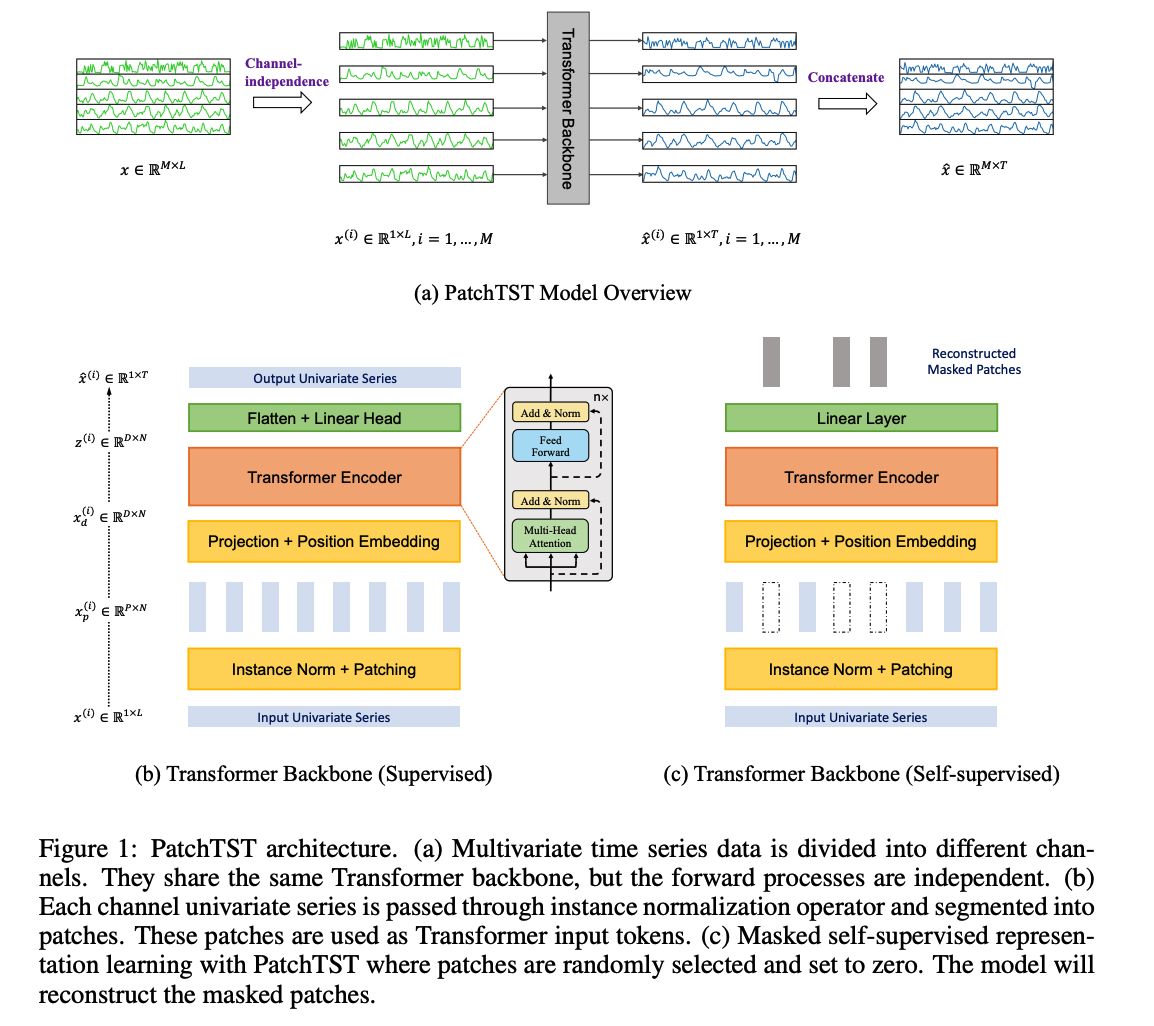
b) Forward Process

\(\boldsymbol{x}_{1: L}^{(i)}=\left(x_1^{(i)}, \ldots, x_L^{(i)}\right)\) : \(i\)-univariate TS of length \(L\)

• where \(i= 1, \cdots M\)

Input : \(\left(\boldsymbol{x}_1, \ldots, \boldsymbol{x}_L\right)\)

• split to \(M\) univariate TS \(\boldsymbol{x}^{(i)} \in \mathbb{R}^{1 \times L}\)

• each of them is fed independently into the Transformer backbone

  ( under channel-independence setting )

Output : \(\hat{\boldsymbol{x}}^{(i)}=\left(\hat{x}_{L+1}^{(i)}, \ldots, \hat{x}_{L+T}^{(i)}\right) \in \mathbb{R}^{1 \times T}\)

• forecasting horizon : \(T\)

c) Patching

Input : univariate time series \(\boldsymbol{x}^{(i)}\)

• divided into patches ( either overlapped or non-overlapped )
  • patch length = \(P\)
  • stride = \(S\)

Output : sequence of patches \(\boldsymbol{x}_p^{(i)} \in \mathbb{R}^{P \times N}\)

• \(N=\left\lfloor\frac{(L-P)}{S}\right\rfloor+2\) : number of patches
• pad \(S\) repeated numbers of the last value \(x_L^{(i)} \in \mathbb{R}\) to the end

Result : number of input tokens can reduce from \(L\) to approximately \(L / S\).

• memory usage & computational complexity of the attention map : quadratically decreased by a factor of \(S\)

d) Loss Function : MSE

Loss in each channel : \(\left\|\hat{\boldsymbol{x}}_{L+1: L+T}^{(i)}-\boldsymbol{x}_{L+1: L+T}^{(i)}\right\|_2^2\)

Total Loss : \(\mathcal{L}=\mathbb{E}_{\boldsymbol{x}} \frac{1}{M} \sum_{i=1}^M\left\|\hat{\boldsymbol{x}}_{L+1: L+T}^{(i)}-\boldsymbol{x}_{L+1: L+T}^{(i)}\right\|_2^2\)

e) Instance Normalization

help mitigating the distribution shift effect ( between the training and testing data )

simply normalizes each time series instance \(\boldsymbol{x}^{(i)}\) with N(0,1)

\(\rightarrow\) normalize each \(\boldsymbol{x}^{(i)}\) before patching & scale back at prediction

(2) Representation Learning

Propose to apply PatchTST to obtain useful representation of the multivariate time series

• via masking & reconstructing

Apply the MTS to transformer ( each input token is a vector \(\boldsymbol{x}_i\) )

Masking : placed randomly within each TS and across different series

2 potential issues

• (1) masking is applied at the level of single time steps
  • masked values : can be easily inferred by interpolating
• (2) design of the output layer for forecasting task can be troublesome
  • parameter matrix \(W\) : \((L \cdot D) \times(M \cdot T)\)
    • \(L\) : time length
    • \(D\) : dimension of \(\boldsymbol{z}_t \in \mathbb{R}^D\) corresponding to all \(L\) time steps
    • \(M\) : TS with \(M\) variable
    • \(T\) : prediction horizon

PatchTST overcome these issues

• Instead of prediction head …. attach \(D \times P\) linear layer
• Instead of overlapping patches …. use non-overlapping patches
  • ensure observed patches do not contain information of the masked ones
  • select a subset of the patch indices uniformly at random

etc )

• trained with MSE loss to reconstruct the masked patches

• each TS will have its own latent representation

  • cross-learned via shared weight
  • allow the pre-training data to contain different # of TS

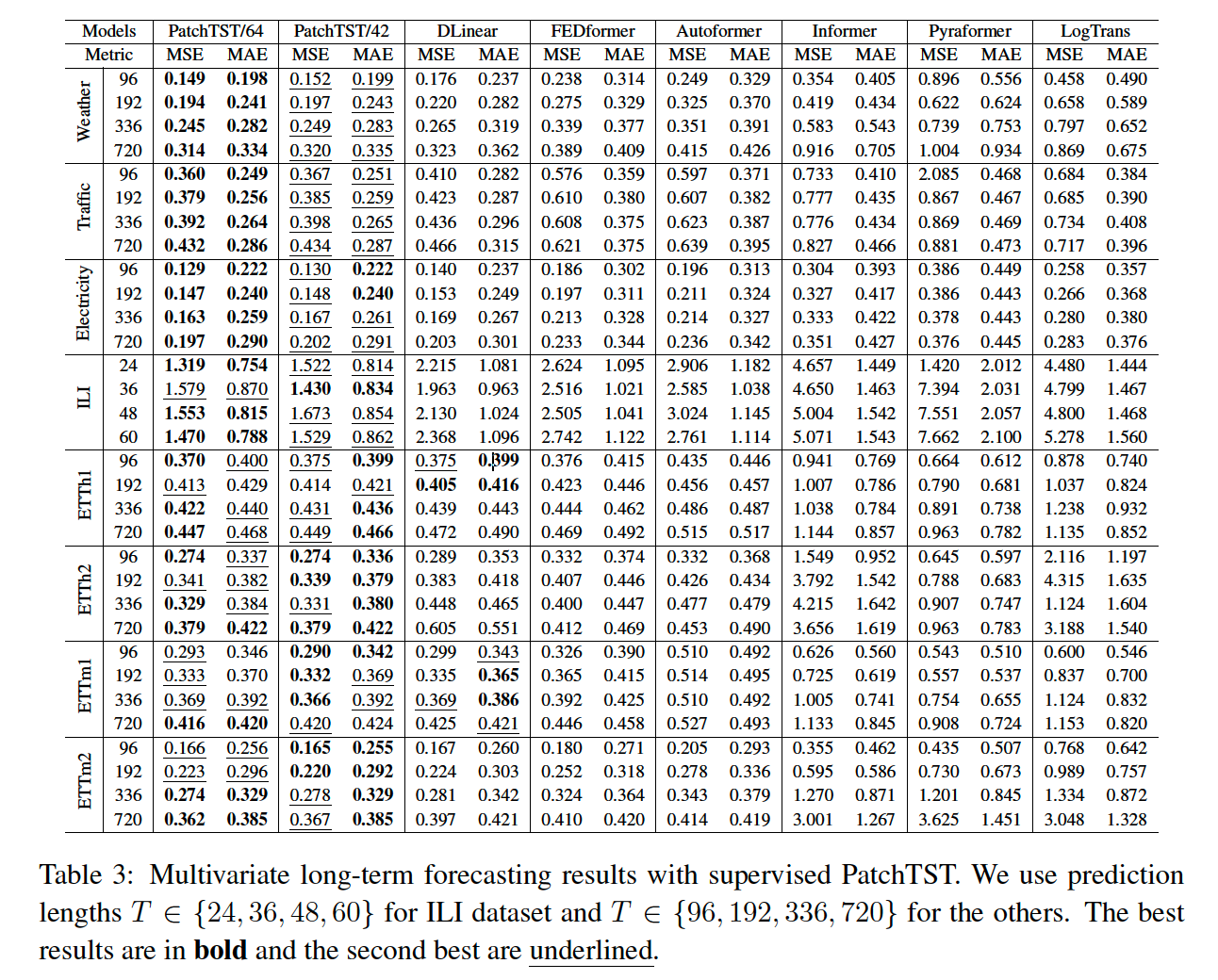
3. Experiments

(1) Long Term TS Forecasting

a) Datasets

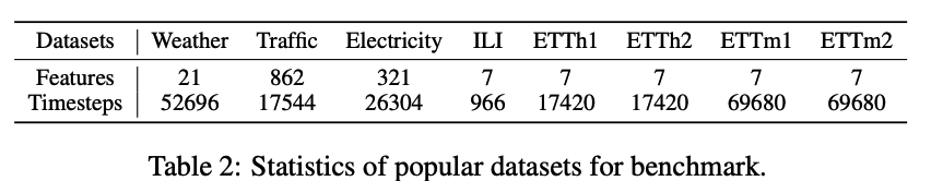
Among these 8 popular datasets..

• several large datasets: Weather, Traffic, and Electricity

  \(\rightarrow\) more stable and less susceptible to overfitting than other smaller datasets.

b) Baselines & Experimental SEttings

Baselines : SOTA Transformer-based models

• same experimental settings

  • prediction length \(T\) :
    • [ILI dataset] 24,36,48,60
    • [others] 96,192,336,720
  • collect baseline from Zeng et al. (2022) ( = Linear/DLinear/NLinear )

• in order to vaoid undersetimating the baselines…

  • also run FEDformer / Autoformer / Informer for 6 different look-back window

    ( L \(\in \{24, 48,96,192,336,720\}\) & chose the best results )

  • more details in Appendix A.1.2

• metrics : MSE & MAE

c) Model Variants

2 versions of PatchTST

• PatchTST/64 :
  • # of input patches = 64
  • look-back window = 512
• PatchTST/42
  • # of input patches = 42
  • look-back window = 336
• for both…
  • patch length \(P\) = 16
  • stride \(S\) = 8

Summary

• PatchTST/42 : for fair comparison
• PatchTST/64 : better reseults for larger datsaets

d) Results

MTS forecasting

UTS forecasting

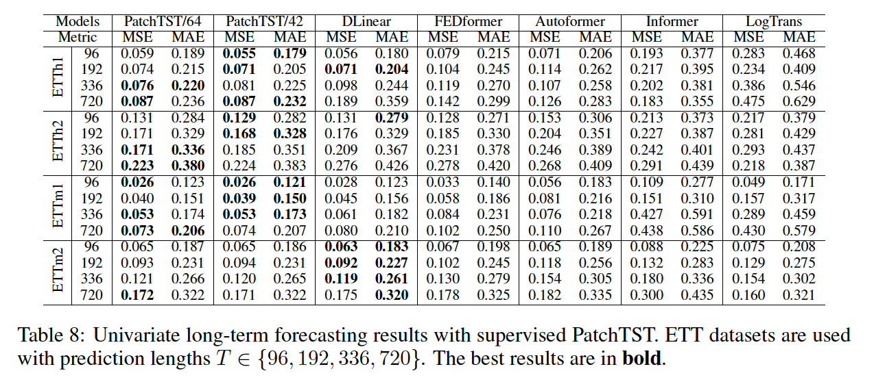
(2) Representation Learning

a) Settings

experiments with masked self-supervised learning

• where we set the patches to be non-overlapped

Settings :

• input sequence length = 512
• patch size = 12 ( thus, 42 patches )
• high masking ratio : 40%
  • mask with zero

Procedure

• Step 1) apply self-supervised pre-training ( 100 epochs )

• Step 2) perform supervised training , with 2 options

  • (a) linear probing

    • only train model head for 20 epochs & freeze rest

  • (b) end-to-end fine-tuning

    • linear probing for 10 epochs to update model head
    • then, end-to-end fine tuning for 20 epochs

    ( proven that a 2-step strategy with linear probing followed by fine-tuning can outperform only doing fine-tuning directly (Kumar et al., 2022) )

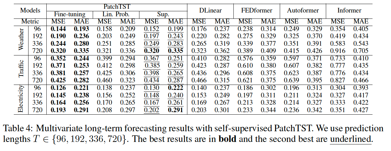
b) Comparison with Supervised methods

performance of PatchTST (ver1,2,3) vs supervised

• ver 1) fine-tuning
• ver 2) linear probing
• ver 3) supervising from scratch

c) Transfer Learning

pre-train the model on Electricity dataset

• fine-tuning MSE is lightly worse than pre-training and fine-tuning on the same dataset
• fine-tuning performance is also worse than supervised training in some cases.
• However, the forecasting performance is still better than other models

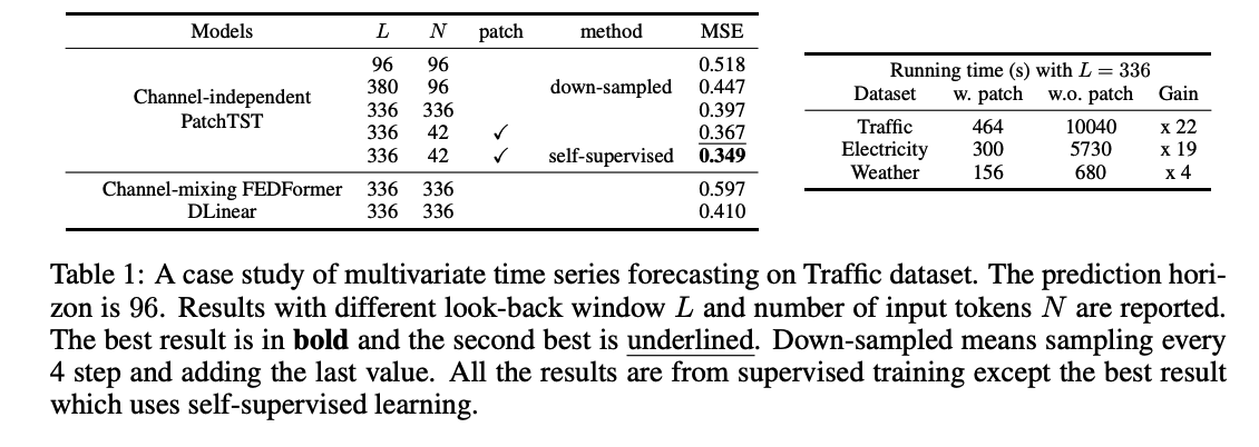
supervised PatchTST

• Entire model is trained for EACH PREDICTION HORIZON

self-supervised PatchTST

• only retrain the linear head or the entire model for much fewer epochs

  \(\rightarrow\) results in significant computational time reduction.

d) Comparison with other SSL methods

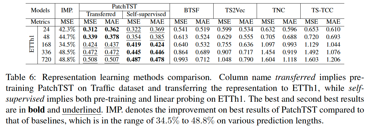
• test the forecasting performance on ETTh1 dataset

• only apply linear probing after the learned representation is obtained (only fine-tune the last linear layer) for fair comparison

( cite results of TS2Vec from (Yue et al., 2022) and {BTSF,TNC,TS-TCC} from (Yang & Hong, 2022) )

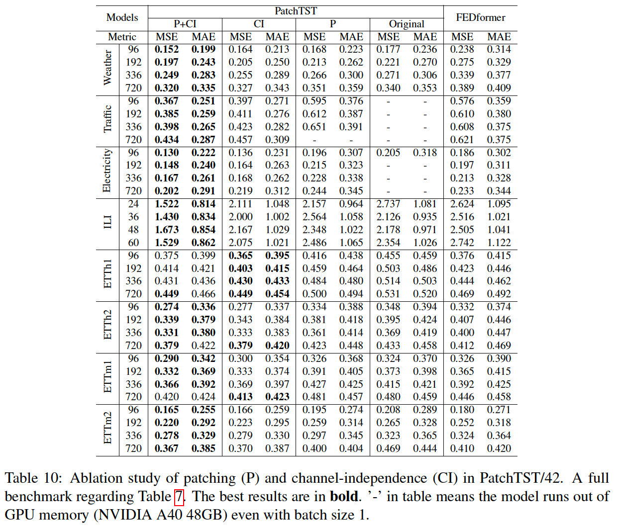
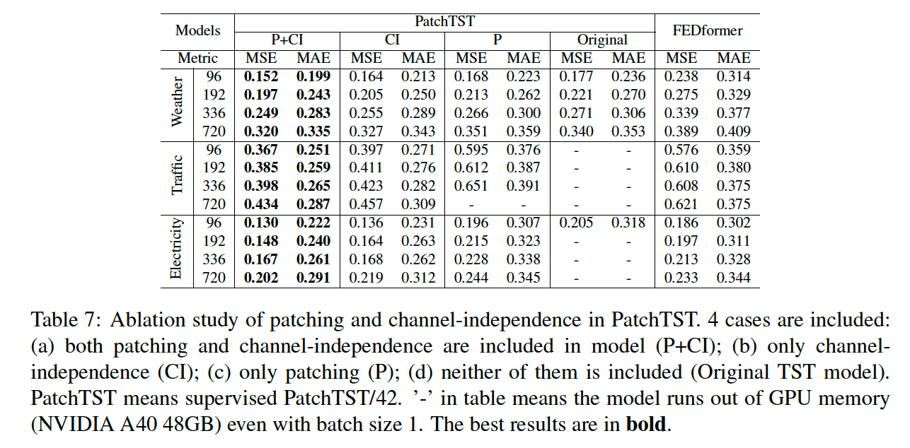
(3) Ablation Study

a) Patching & Channel Independence

with /w.o patching / channel-independence

both of them are important factors

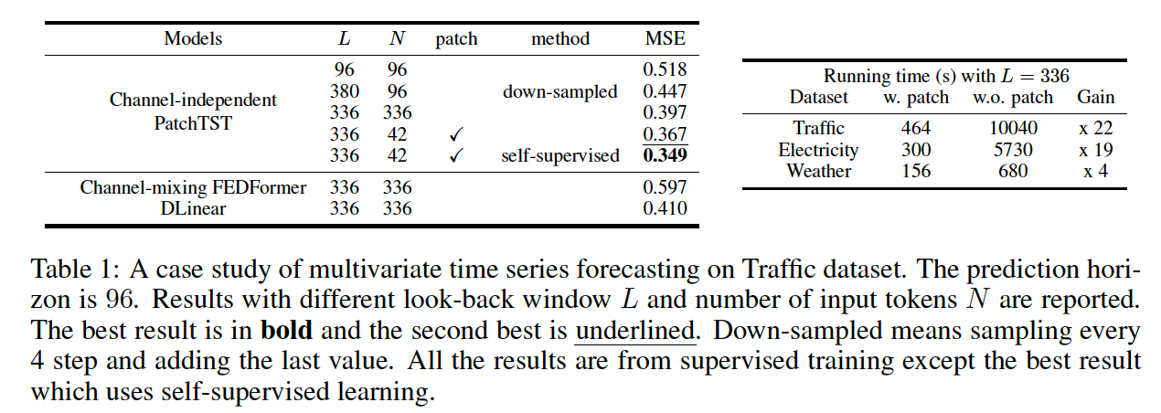
Patching

• motivation of patching is natural
• improves the running time and memory consumption
  • due to shorter Transformer sequence input.

Channel-independence

• may not be intuitive

• provide an in-depth analysis on the key factors that make channel-independence more preferable in Appendix A.7.

  • (1) Adaptability: Since each time series is passed through the Transformer separately, it generates its own attention maps. That means different series can learn different attention patterns for their prediction, as shown in Figure 6. In contrast, with the channel mixing approach, all the series share the same attention patterns, which may be harmful if the underlying multivariate time series carries series of different behaviors.
  • (2) Channel-mixing models may need more training data to match the performance of the channelindependent ones. The flexibility of learning cross-channel correlations could be a doubleedged sword, because it may need much more data to learn the information from different channels and different time steps jointly and appropriately, while channel-independent models only focus on learning information along the time axis.
  • (3) Channel-independent models are less likely to overfit data during training.

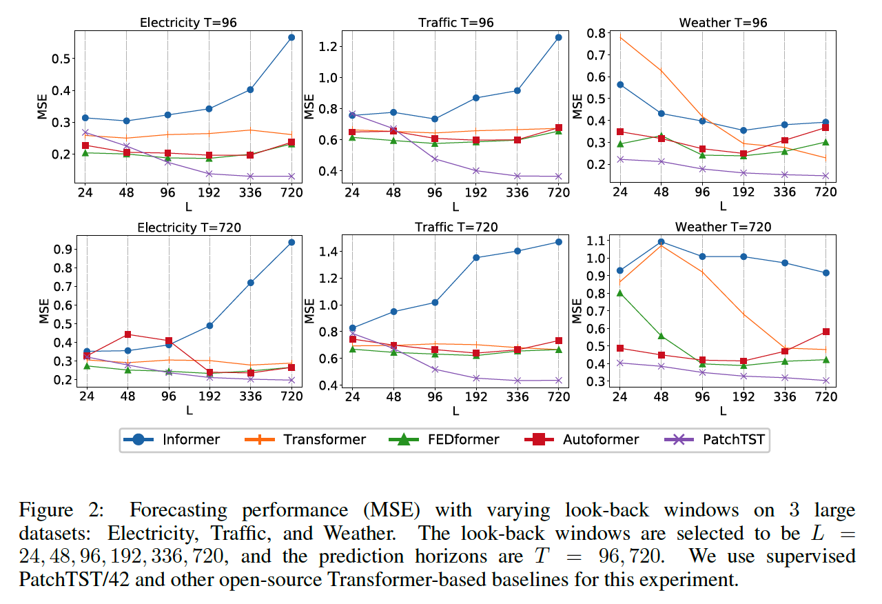
b) Varying Look-back Window

longer look-back window increases the receptive field,

\(\rightarrow\) potentially improves the forecasting performance.

However…

• (1) as argued in (Zeng et al., 2022), this phenomenon hasn’t been observed in most of the Transformer-based models.
• (2) demonstrate in Figure 2 that in most cases, these Transformer-based baselines have not benefited from longer look-back window \(L\)
  • which indicates their ineffectiveness in capturing temporal information.

PatchTST : consistently reduces the MSE scores as the receptive field increases

4. Conclusion

Proposes an effective design of Transformer-based models for time series forecasting tasks

Introducing 2 key components:

• (1) patching
  • simple but proven tobe an effective operator that can be transferred easily to other models
• (2) channel-independent structure
  • can be further exploited to incorporate the correlation between different channels

Benefits

• capture local semantic information
• benefit from longer look-back windows

Experiments

• outperforms other baselines in supervised learning,
• prove its promising capability in self-supervised representation learning & transfer learning.