(paper 76) CrossFormer; Transformer Utilizing Cross-dimension Dependency for MTS Forecasting

CrossFormer: Transformer Utilizing Cross-dimension Dependency for MTS Forecasting

Contents

1. Abstract
2. Introduction
3. Related Works
   1. MTS forecasting
   2. Transformers for MTS forecasting
   3. Vision Transformers
4. Methodology
   1. Dimension-Segment-Wise Embedding
   2. Two-Stage Attention Layer
   3. Hierarchical Encoder-Decoder
5. Experiments
   1. Main Results
   2. Ablation Study

0. Abstract

MTS forecasting

• Transformer-based models : can capture long-term dependency

\(\rightarrow\) however … mainly focus on modeling the temporal (cross-time) dependency

( omit the dependency among different variables ( = cross-dimension dependency ) )

Propose Crossformer

• Transformer-based model utilizing cross-dimension dependency for MTS forecasting.

Details:

• (step 1) Input MTS is embedded into a 2D vector array

  • via Dimension-Segment-Wise (DSW) embedding

    ( to preserve time and dimension information )

• (step 2) Two-Stage Attention (TSA) layer

  • efficiently capture the cross-time & cross-dimension dependency

using both DSW & TSA, Crossformer establishes a Hierarchical Encoder-Decoder (HED) to use the information at different scales for the final forecasting

1. Introduction

Transformer for MTS forecasting:

• ability to capture long-term temporal dependency (cross-time dependency).

Cross-dimension dependency is also critical for MTS forecasting !

• ex) previous neural models : explicitly capture the cross-dimension dependency, using CNN/GNN

• However, recent Transformer-based models …

  \(\rightarrow\) only implicitly utilize this dependency by embedding

  • generally embed data points in all dimensions at the same time step into a feature vector

    & try to capture dependency among different time steps (Fig. 1 (b))

    \(\rightarrow\) cross-time dependency is well captured, but cross-dimension dependency is not

Crossformer

a Transformer-based model that explicitly utilizes cross-dimension dependency for MTS forecasting.

• (1) Dimension-Segment-Wise (DSW) embedding

  • to process the historical time series.

  • step 1) series in each dimension is partitioned into segments

  • step 2) embedded into feature vectors

    ( output = 2D vector array … two axes = time & dimension )

• (2) Two-Stage-Attention (TSA) layer

  • efficiently capture the cross-time & cross-dimension dependency

\(\rightarrow\) using (1) & (2) … establishes a Hierarchical Encoder-Decoder (HED)

• each layer = each scale

• [Encoder] upper layer = merges adjacent segments output by the lower layer

  ( capture coarser scale )

• [Decoder] generate predictions at different scales & add them up as the final prediction.

Contribution

• existing Transformer-based models : cross-dimension dependency is not well utilized

  \(\rightarrow\) Without adequate and explicit mining and utilization of cross-dimension dependency, their forecasting capability is empirically shown limited.

• develop Crossformer

• extensive epperimental results

2. Related Works

(1) MTS forecasting

Divided into (1) statistical & (2) neural models

a) Statistical

• Vector auto-regressive (VAR) model
• Vector auto-regressive moving average (VARMA)

\(\rightarrow\) assume linear cross-dimension & cross-time dependency.

b) Neural models

• TCN (Lea et al., 2017) & DeepAR (Flunkert et al., 2017)
  • treat the MTS data as a sequence of vectors and use CNN/RNN to capture the temporal dependency
• LSTnet (Lai et al., 2018)
  • CNN : for cross-dimension dependency
  • RNN : for cross-time dependency
• GNNs
  • to capture the cross-dimension dependency explicitly for forecasting
  • ex) MTGNN (Wu et al., 2020) :
    • temporal convolution : cross-time
    • graph convolution : cross-dimension

\(\rightarrow\) capture the cross-time dependency through CNN or RNN … difficulty in modeling long-term dependency

(2) Transformers for MTS forecasting

LogTrans (Li et al., 2019b)

• proposes the LogSparse attention ( reduces the computation complexity )
  • from \(O\left(L^2\right)\) to \(O\left(L(\log L)^2\right)\)

Informer (Zhou et al., 2021)

• utilizes the sparsity of attention score through KL divergence estimation
• proposes ProbSparse self-attention
  • achieves \(O(L \log L)\) complexity.

Autoformer (Wu et al., 2021a)

• introduces a decomposition architecture with an Auto-Correlation mechanism
  • achieves the \(O(L \log L)\) complexity.

Pyraformer (Liu et al., 2021a)

• pyramidal attention module
• summarizes features at different resolutions & models the temporal dependencies of different ranges
  • complexity of \(O(L)\).

FEDformer (Zhou et al., 2022)

• have a sparse representation in frequency domain
• develop a frequency enhanced Transformer
  • \(O(L)\) complexity.

Preformer (Du et al., 2022)

• divides the embedded feature vector sequence into segments
• utilizes segment-wise correlation-based attention

\(\rightarrow\) These models mainly focus on reducing the complexity of cross-time dependency modeling,

but omits the **cross-dimension dependency

(3) Vision Transformers

**ViT (Dosovitskiy et al., 2021) **

• one of the pioneers of vision transformers.

• Basic idea of ViT

  • split an image into non-overlapping medium-sized patches

  • rearranges these patches into a sequence ( to be input to the Transformer )

Idea of partitiong images into patches

\(\rightarrow\) inspires our DSW embedding where MTS is split into dimension-wise segments

Swin Transformer (Liu et al., 2021b)

• performs local attention within a window ( to reduce the complexity )
• builds hierarchical feature maps by merging image patches

3. Methodology

Notation

• future value : \(\mathbf{x}_{T+1: T+\tau} \in\) \(\mathbb{R}^{\tau \times D}\)
• input value : \(\mathbf{x}_{1: T} \in \mathbb{R}^{T \times D}\)
• number of dimension : \(D>1\)

Section 3.1

• embed the MTS using Dimension-Segment-Wise (DSW) embedding
• To utilize the cross-dimension dependency

Section 3.2

• propose a Two-Stage Attention (TSA) layer
• to efficiently capture the dependency among the embedded segments

Section 3.3

• construct a hierarchical encoder-decoder (HED), using DSW embedding and TSA layer
• to utilize information at different scales

(1) Dimension-Segment-Wise Embedding

Embedding of the previous Transformer-based models for MTS forecasting ( Fig. 1 (b) )

• step 1) Embed data points at the same time step into a vector: \(\mathbf{x}_t \rightarrow \mathbf{h}_t, \mathbf{x}_t \in \mathbb{R}^D, \mathbf{h}_t \in \mathbb{R}^{d_{\text {model }}}\),
  • \(\mathbf{x}_t\) : all the data points in \(D\) dimensions at step \(t\).
  • input \(\mathbf{x}_{1: T}\) is embedded into \(T\) vectors \(\left\{\mathbf{h}_1, \mathbf{h}_2, \ldots, \mathbf{h}_T\right\}\).
• step 2) Dependency among the \(T\) vectors is captured for forecasting.

\(\rightarrow\) preivous methods mainly capture cross-time dependency

( cross-dimension dependency is not explicitly captured during embedding )

Fig. 1 (a)

• typical attention score map of original Transformer
• attention values have a tendency to segment, i.e. close data points have similar attention weights.

\(\rightarrow\) Argue that an embedded vector should represent a series segment of single dimension (Fig. 1 (c)), rather than the values of all dimensions at single step (Fig. 1 (b)).

propose Dimension-Segment-Wise (DSW) embedding

[ Step 1 ] Points in each dimension are divided into segments of length \(L_{s e g}\)

\(\begin{aligned} \mathbf{x}_{1: T} & =\left\{\mathbf{x}_{i, d}^{(s)} \mid 1 \leq i \leq \frac{T}{L_{\text {seg }}}, 1 \leq d \leq D\right\} \\ \mathbf{x}_{i, d}^{(s)} & =\left\{x_{t, d} \mid(i-1) \times L_{\text {seg }}<t \leq i \times L_{\text {seg }}\right\} \end{aligned}\).

• where \(\mathbf{x}_{i, d}^{(s)} \in \mathbb{R}^{L_{\text {seg }}}\) is the \(i\)-th segment in dimension \(d\) with length \(L_{\text {seg }}\).

[ Step 2 ] Each segment is embedded into a vector

• using linear projection added with a position embedding

• \(\mathbf{h}_{i, d}=\mathbf{E} \mathbf{x}_{i, d}^{(s)}+\mathbf{E}_{i, d}^{(p o s)}\).

  • \(\mathbf{E} \in \mathbb{R}^{d_{\text {model }} \times L_{\text {seg }}}\) : the learnable projection matrix
  • \(\mathbf{E}_{i, d}^{(\text {pos })} \in \mathbb{R}^{d_{\text {model }}}\) : the learnable position embedding for position \((i, d)\).

[ Output ] obtain a \(2 \mathrm{D}\) vector array \(\mathbf{H}=\left\{\mathbf{h}_{i, d} \mid 1 \leq i \leq \frac{T}{L_{\text {seg }}}, 1 \leq d \leq D\right\}\),

• each \(\mathbf{h}_{i, d}\) represents a univariate time series segment.

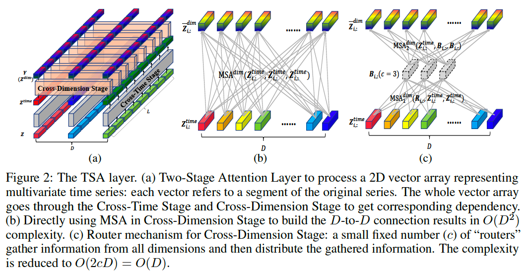
(2) Two-Stage Attention Layer

Flatten 2D array \(\mathbf{H}\) into 1D sequence

\(\rightarrow\) to be input to Trarnsformer architecture

Specific considerations:

• (1) Different from images where the axes of height and width are interchangeable……

  the axes of time and dimension for MTS have different meanings and thus should be treated differently

• (2) Directly applying self-attention on \(2 \mathrm{D}\) array will cause the complexity of \(O\left(D^2 \frac{T^2}{L_{s e g}^2}\right)\) …..

  which is unaffordable for large \(D\).

\(\rightarrow\) propose the Two-Stage Attention (TSA) Layer

• to capture cross-time and cross-dimension dependency

a) Cross-Time stage

Notation

• Input : 2D array \(\mathbf{Z} \in \mathbb{R}^{L \times D \times d_{\text {model }}}\)

  ( = output of DSW embedding or lower TSA layers )

  • \(L\) : number of segments
  • \(D\): number of dimensions

• \(\mathbf{Z}_{i,:}\) : vectors of all dimensions at time step \(i\)

• \(\mathbf{Z}_{:, d}\) : vectors of all time steps in dimension \(d\).

Multi-head self-attention (MSA) to each dimension:

\(\begin{aligned} \hat{\mathbf{Z}}_{:, d}^{\text {time }} & =\text { LayerNorm }\left(\mathbf{Z}_{:, d}+\operatorname{MSA}^{\text {time }}\left(\mathbf{Z}_{:, d}, \mathbf{Z}_{:, d}, \mathbf{Z}_{:, d}\right)\right) \\ \mathbf{Z}^{\text {time }} & =\operatorname{LayerNorm}\left(\hat{\mathbf{Z}}^{\text {time }}+\operatorname{MLP}\left(\hat{\mathbf{Z}}^{\text {time }}\right)\right) \end{aligned}\).

• where \(1 \leq d \leq D\)
• all dimensions \((1 \leq d \leq D)\) share the same MSA layer

Computation complexity of cross-time stage = \(O\left(D L^2\right)\).

Dependency among time segments in the same dimension is captured in \(\mathbf{Z}^{\text {time }}\).

\(\rightarrow\) \(\mathbf{Z}^{\text {time }}\) becomes the input of Cross-Dimension Stage

b) Cross-Dimension stage

Cross-Time stage

• we can use a large \(L_{\text {seg }}\) for long sequence in DSW Embedding

  ( to reduce the number of segments \(L\) in cross-time stage )

Cross-Dimension Stage

• we can not partition dimensions and directly apply MSA

• Instead, we propose the router mechanism for potentially large \(D\).

  • set a small fixed number \((c<<D)\) of learnable vectors for each time step \(i\) as routers.
  • complexity : \(O(D^2L) \rightarrow O(DL)\)

• Routers

  • step 1) aggregate messages from all dimensions
  • step 2) distribute the received messages among dimensions

  \(\rightarrow\) all-to-all connection among \(D\) dimensions are built:

\(\begin{aligned} \mathbf{B}_{i,:} & =\operatorname{MSA}_1^{d i m}\left(\mathbf{R}_{i,:}, \mathbf{Z}_{i,:}^{\text {time }}, \mathbf{Z}_{i,:}^{\text {time }}\right), 1 \leq i \leq L \\ \overline{\mathbf{Z}}_{i,:}^{d i m} & =\operatorname{MSA}_2^{d i m}\left(\mathbf{Z}_{i,:}^{\text {time }}, \mathbf{B}_{i,:}, \mathbf{B}_{i,:}\right), 1 \leq i \leq L \\ \hat{\mathbf{Z}}^{\text {dim }} & =\text { LayerNorm }\left(\mathbf{Z}^{\text {time }}+\overline{\mathbf{Z}}^{\text {dim }}\right) \\ \mathbf{Z}^{\text {dim }} & =\text { LayerNorm }\left(\hat{\mathbf{Z}}^{\text {dim }}+\operatorname{MLP}\left(\hat{\mathbf{Z}}^{d i m}\right)\right) \end{aligned}\).

• \(\mathbf{R} \in \mathbb{R}^{L \times c \times d_{\text {model }}}\) : learnable vector array ( = routers )
• \(\mathbf{B} \in \mathbb{R}^{L \times c \times d_{\text {model }}}\) : aggregated messages from all dimensions
• \(\overline{\mathbf{Z}}^{\text {dim }}\) : output of the router mechanism.
• \(\hat{\mathbf{Z}}^{\text {dim }}\) : output of skip connection
• \(\mathbf{Z}^{\text {dim }}\) : output of MLP

All time steps \((1 \leq i \leq L)\) share the same \(\mathrm{MSA}_1^{d i m}, \mathrm{MSA}_2^{\text {dim }}\).

\(\mathbf{Y}=\mathbf{Z}^{\text {dim }}=\mathrm{TSA}(\mathbf{Z})\).

• \(\mathbf{Z}\) : input vector array of TSA layer
• \(\mathbf{Y} \in \mathbb{R}^{L \times D \times d_{\text {model }}}\) : output vector array of TSA layer

Overall computation complexity of TSA layer

• \(O\left(D L^2+D L\right)=O\left(D L^2\right)\).

Summary

After the Cross-Time and Cross-Dimension Stages …

every two segments (i.e. \(\mathbf{Z}_{i_1, d_1}, \mathbf{Z}_{i_2, d_2}\) ) in \(\mathbf{Z}\) are connected,

\(\rightarrow\) both cross-time and cross-dimension dependencies are captured in \(\mathbf{Y}\).

(3) Hierarchical Encoder-Decoder

to capture information at different scales

use (1) DSW embedding & (2) TSA layer & (3) segment merging

\(\rightarrow\) to construct a Hierarchical Encoder-Decoder (HED).

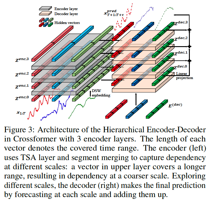
• Upper layer utilizes information at a coarser scale for forecasting.
• Final results = add forecasting values at different scales

a) Encoder

Coarser Level : every two adjacent vectors in time domain are merged

\(\rightarrow\) then, TSA layer is applied to capture dependency at this scale.

\(\mathbf{Z}^{e n c, l}=\operatorname{Encoder}\left(\mathbf{Z}^{e n c, l-1}\right)\).

Details :

\(\begin{aligned} & \left\{\begin{aligned} l=1: & \hat{\mathbf{Z}}^{e n c, l}=\mathbf{H} \\ l>1: & \hat{\mathbf{Z}}_{i, d}^{e n c, l}=\mathbf{M}\left[\mathbf{Z}_{2 i-1, d}^{e n c, l-1} \cdot \mathbf{Z}_{2 i, d}^{e n c, l-1}\right], 1 \leq i \leq \frac{L_{l-1}}{2}, 1 \leq d \leq D \end{aligned}\right. \\ & \mathbf{Z}^{e n c, l}=\operatorname{TSA}\left(\hat{\mathbf{Z}}^{e n c, l}\right) \\ & \end{aligned}\).

• \(\mathbf{H}\) : \(2 \mathrm{D}\) array obtained by DSW embedding
• \(\mathbf{Z}^{\text {enc,l }}\) : the output of the \(l\)-th encoder layer
• \(\mathbf{M} \in \mathbb{R}^{d_{\text {model }} \times 2 d_{\text {model }}}\) : a learnable matrix for segment merging
• \(L_{l-1}\) : the number of segments in each dimension in layer \(l-1\)
• \(\hat{\mathbf{Z}}^{e n c, l}\) : the array after segment merging in the \(i\)-th layer.

Suppose there are \(N\) layers in the encoder

\(\rightarrow\) use \(\mathbf{Z}^{\text {enc }, 0}, \mathbf{Z}^{\text {enc,1 }}, \ldots, \mathbf{Z}^{\text {enc, }, N},\left(\mathbf{Z}^{\text {enc }, 0}=\mathbf{H}\right)\) to represent the \(N+1\) outputs of the encoder.

• complexity of each encoder layer : \(O\left(D \frac{T^2}{L_{\text {seg }}^2}\right)\).

b) Decoder

Output of encoder : \(N+1\) feature arrays

Layer \(l\) of decoder :

• Input : \(l\)-th encoded array
• Output : decoded \(2 \mathrm{D}\) array of layer \(l\).

Summary : \(\mathbf{Z}^{\text {dec }, l}=\operatorname{Decoder}\left(\mathbf{Z}^{\text {dec }, l-1}, \mathbf{Z}^{\text {enc }, l}\right)\) :

Linear projection is applied to each layer’s output

• to yield the prediction of each layer

Layer predictions

• summed to make the final prediction (for \(l=0, \ldots, N\) ):

\(\begin{gathered} \text { for } l=0, \ldots, N: \mathbf{x}_{i, d}^{(s), l}=\mathbf{W}^l \mathbf{Z}_{i, d}^{\text {dec, }, l} \quad \mathbf{x}_{T+1: T+\tau}^{\text {pred,l }}=\left\{\mathbf{x}_{i, d}^{(s), l} \mid 1 \leq i \leq \frac{\tau}{L_{\text {seg }}}, 1 \leq d \leq D\right\} \\ \mathbf{x}_{T+1: T+\tau}^{\text {pred }}=\sum_{l=0}^N \mathbf{x}_{T+1: T+\tau}^{\text {pred, }} \end{gathered}\).

• \(\mathbf{W}^l \in \mathbb{R}^{L_{s e g} \times d_{\text {model }}}\) : a learnable matrix to project a vector to a time series segment.
• \(\mathbf{x}_{i, d}^{(s), l} \in \mathbb{R}^{L_{s e g}}\) : the \(i\)-th segment in dimension \(d\) of the prediction

4. Experiments

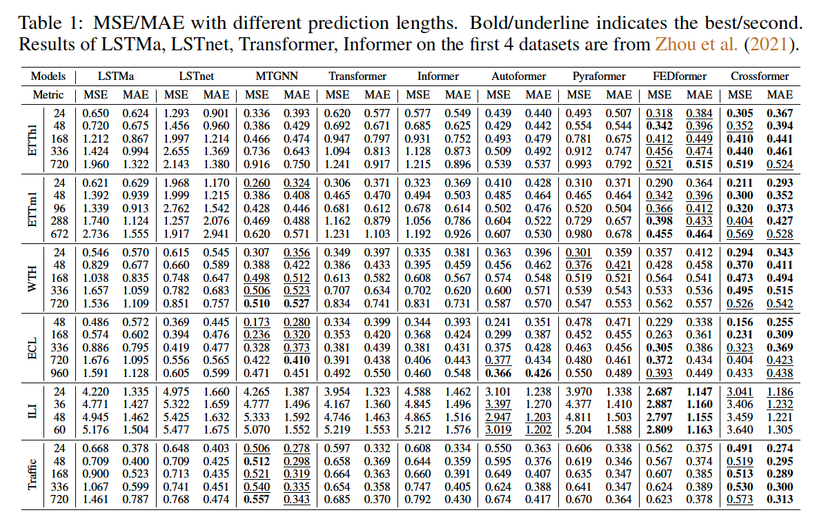
(1) Main Results

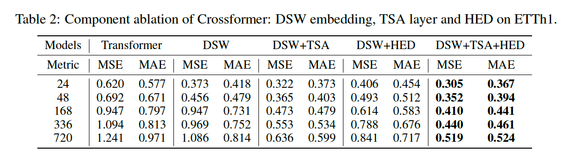
(2) Ablation Study