(paper 88) Novel Class Discovery; an Introduction and Key Concepts

Novel Class Discovery: an Introduction and Key Concepts

Contents

1. Abstract
2. Introduction

0. Abstract

Novel Class Discovery (NCD)

• labeled set of KNOWN classes & unlabeled set of UNKNOWN classes

Comprehensive survey of the NCD

• (1) Define the NCD problem

• (2) Overview of the different families of approaches

  • By how they transfer knowledge from the labeled \(\rightarrow\) unlabeled

    ( either learn in 2 stages )

    • (1) Extracting knowledge from the labeled data only & applying it to the unlabeled data
    • (2) Conjointly learning on both sets.

• (3) Introduce some new related tasks

• (4) Present some common tools and techniques used in NCD

  • ex) pseudo labeling, SSL, CL

1. Introduction

Real World Problems :

\(\rightarrow\) Not always possible to have labeled data for all classes of interest

Open-world Assumption : Instances outside the initial set of classes may emerge

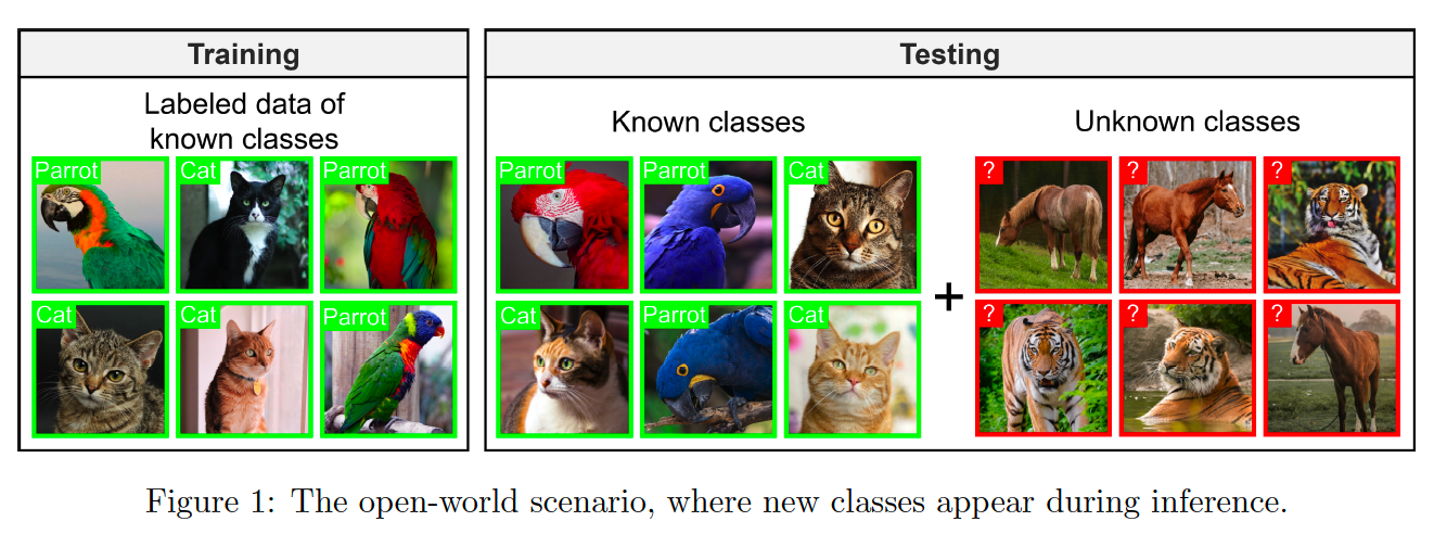
• Instances from classes never seen during training appear at test time
• Ideal model : should classify all cases!

What is the issue?

Standard classification model

• incorrectly classify instances that fall outside the known classes as belonging to one of the known classes.

  \(\rightarrow\) produce overconfident incorrect predictions

Researchers are now exploring scenarios where unlabeled data is also available

Setting of this paper :

where a labeled set of known classes and an unlabeled set of unknown classes are given during training.

Goal : learn to categorize the unlabeled data into the appropriate classes.

\(\rightarrow\) “Novel Class Discovery (NCD)”

What is the usual setup of NCD?

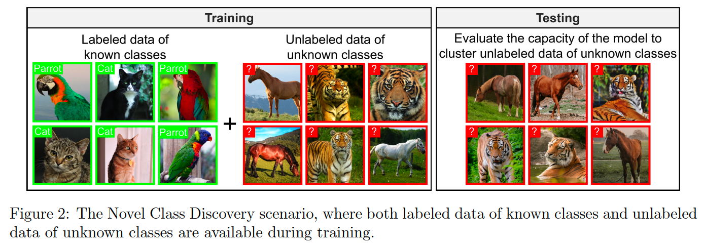
Training data :

• (1) from known classes
• (2) from unknown classes

Test set :

• only samples from unknown classes.

NCD scenario belongs to Weakly Supervised Learning

• manage classes that have never appeared during training
• ex) Open-World Learning (OWL)
• ex) Zero-Shot Learning (ZSL)

Open-World Learning (OWL)

• seek to accurately label samples of classes seen during training,

  while identifying samples from unknown classes.

• BUT not tasked with clustering the unknown classes

  ( + unlabeled data is left unused )

Zero-Shot Learning (ZSL)

• designed to accurately predict classes that have never appeared during training.

  ( still… some kind of description of these unknown classes is needed to be able to recognize them )

\(\leftrightarrow\) NCD has recently gained significant attention due to its practicality and real-world applications.

Why does clustering alone fail to produce good results?

Clustering is a direct solution to the NCD problem

Many clustering methods have obtained an accuracy larger than \(90 \%\) on the MNIST dataset

( \(\leftrightarrow\) but not in complex datasets )

Clustering can fail due to the assumptions of…

• spherical clusters, mixture of Gaussian distributions, shape of the data, similarity measure, etc.

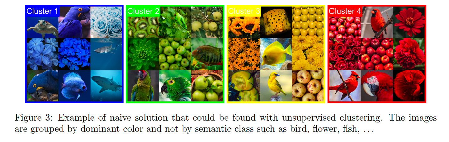
• Although the clusters formed in this manner will be statistically accurate,

  the semantic categories will not be revealed!

Need for more refined techniques that can extract from known classes a relevant representation of a class in order to improve the clustering process.

To fill these gaps

Novel Class Discovery

• identify new classes in unlabeled data by exploiting prior knowledge from known classes.

• key idea )

  • by having a set of known classes, should be able to improve its performance by extracting a general concept of what constitutes a good class.

  • assumed that the model does not need to be able to distinguish the known from the unknown classes.

    ( \(\leftrightarrow\) Generalized Category Discovery (GCD) )

Difficulty of a NCD problem :

\(\rightarrow\) is set by varying the number of known/unknown classes

• increase in known class = EASIER task

Influence of the semantic similarity between

• (1) classes of the labeled sets
• (2) classes of the unlabeled sets

\(\rightarrow\) if HIGH similarity, EASIER task

( + LOW semantic similarity : can even have a negative impact )

Contributions and Organization

Detailed overview of Novel Class Discovery

Outline the key components present in most NCD methods

• organized by the way they transfer knowledge from the labeled to the unlabeled set.

Related works in the context of NCD

2. Preliminaries

(1) A brief history of NCD

2018 article of Hsu et al. [5]

• transfer learning task where the labels of the target set are not available and must be inferred.
• Methods : KCL & MCL
  • still regularly used

“Novel Category Discovery”

• used by Han et al. [18] in 2020
• on this work, Zhong et al. defined “Novel Class Discovery”

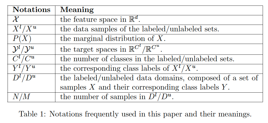
(2) A formal definition of NCD

During training, the data is provided in two distinct sets, a

Notation

• labeled set \(D^l=\left\{\left(x_i^l, y_i^l\right)\right\}_{i=1}^N\)
• unlabeled set \(D^u=\left\{x_i^u\right\}_{i=1}^M\).

Goal : use both \(D^l\) and \(D^u\) to discover the \(C^u\) novel classes

• usually done by partitioning \(D^u\) into \(C^u\) clusters and associating labels \(y_i^u \in \mathcal{Y}^u=\left\{1, \ldots, C^u\right\}\) to the data in \(D^u\).

Settings

• No overlap between the classes of \(\mathcal{Y}^l\) and \(\mathcal{Y}^u\) ( \(\mathcal{Y}^l \cap \mathcal{Y}^u=\emptyset\). )
• Not concerned with the accuracy on the classes of \(D^l\),
• Most works : the number of novel classes \(C^u\) is assumed to be KNOWN
  • some works attempt to estimate this number.

(3) Positioning and key concepts of NCD

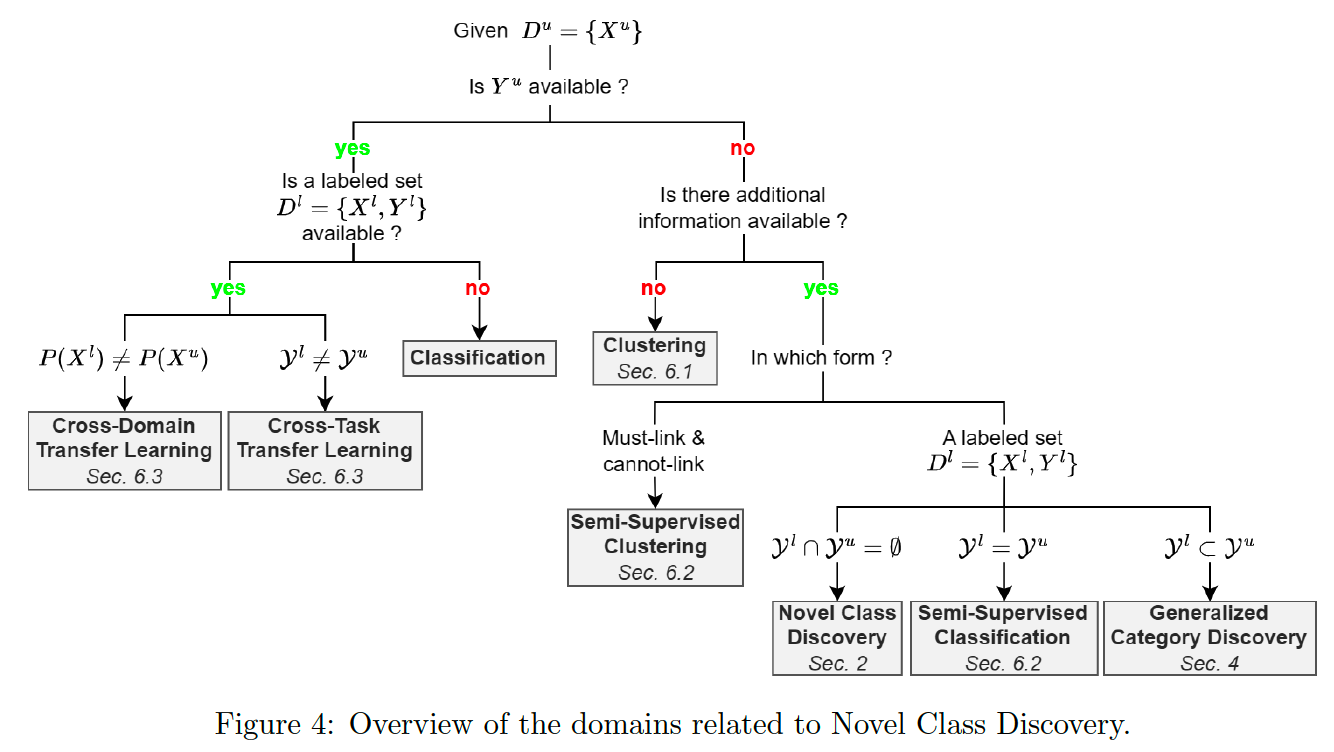
( Open World Learning is reviewed in Section 6.4 but does not appear in this figure. )

(4) Evaluation protocol & metrics in NCD

How to set unlabeled dataset ??

• hold out during the training phase a portion of the classes ( from a fully labeled dataset )

  \(\rightarrow\) treat them as novel classes & form the unlabeled dataset \(D^u\).

• ex) MNIST

  • 0~4 : known classes
  • 5~9 : unknown classes

Performance metrics

• only computed on \(D^u\)

a) Clustering accuracy (ACC)

• requires to optimally map the predicted labels to the GT labels

  ( \(\because\) cluster numbers won’t necessarily match the class numbers )

• can be obtained with the the Hungarian algorithm

\(A C C=\frac{1}{M} \sum_{i=1}^M \mathbb{1}\left[y_i^u=\operatorname{map}\left(\hat{y}_i^u\right)\right]\).

• \(\operatorname{map}\left(\hat{y}_i^u\right)\) : the mapping of the predicted label for sample \(x_i^u\)
• \(M\) : number of samples in the unlabeled set \(D^u\).

b) Normalized mutual information (NMI)

• correspondence between the predicted and ground-truth labels
• invariant to permutations

\(N M I=\frac{I\left(\hat{y}^u, y^u\right)}{\sqrt{H\left(\hat{y}^u\right) H\left(y^u\right)}}\).

• \(I\left(\hat{y}^u, y^u\right)\) : mutual information between \(\hat{y}^u\) and \(y^u\)
• \(H\left(y^u\right)\) and \(H\left(\hat{y}^u\right)\) : marginal entropies of the empirical distributions of \(y^u\) and \(\hat{y}^u\) respectively.

c) Summary

Both ACC & NMI : range between 0 and 1

• closer to 1, the better

Other metrics

• Balanced Accuracy (BACC) and the Adjusted Rand Index (ARI).

  • BACC : for imbalanced class distribution

    ( = calculated as the average of sensitivity and specificity )

  • ARI : normalized measure of agreement between the predicted clusters & GT

    ( ranges from -1 ~ 1 …. 0 = random clustering )

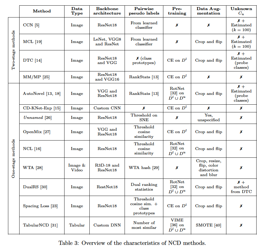
3. Taxonomy of NCD methods

NCD : organized by the way in which they transfer knowledge

• from the labeled set \(D^l\) to the unlabeled set \(D^u\).

Adopt either a one or two-stage approach.

Two-stage approaches

Tackle the NCD problem in a way similar to cross-task Transfer Learning (TL)

• step 1) focus on \(D^l\) only
  • Two families of methods :
    • (1) Uses \(D^l\) to learn a similarity function
    • (2) Incorporates the features relevant to the classes of \(D^l\) into a latent representation.
• step 2) transfer to \(D^{u}\)

One-stage apprroaches

Process \(D^l\) and \(D^u\) simultaneously

• using a shared objective function.

Latent space shared by \(D^l\) and \(D^u\)

• trained by 2 classification networks with different objectives.

• ex) unlabeled : clustering & labeled : accuracy ( classification )

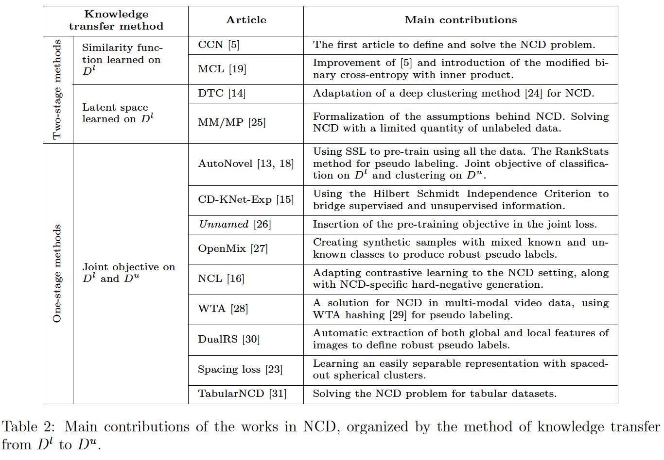
(1) Two-stage methods

a) Learned-similaity-based

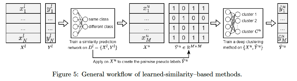
Step 1) Learning function on \(D^l\) ( that is also applicable on \(D^u\) )

• determines if pairs of instances belong to the same class or not

• \(C^l\) and \(C^u\) of classes can be different !

\(\rightarrow\) Binary classification network is generally trained from the existing class labels \(Y^l\).

Step 2) Learned function is then applied on each unique pair of instances in the unlabeled set \(D^u=\left\{X^u\right\}\)

• form a pairwise pseudo label matrix \(\tilde{Y}^u\).

  ( use this pseudo label as target )

• Train a classifier on \(D^u\) & pseudo-label

[ Constrained Clusteing Network (CCN) ]

Tackles the

• cross-domain TL problem
• cross-task TL problem ( = NCD )
  • seeks to cluster \(D^u\) by using the knowledge of a network trained on \(D^l\). I

Step 1) Similarity prediction network is trained on \(D^l\)

• whether they are from the same class

Step 2) Apply it on \(D^u\)

• create a matrix of pairwise pseudo labels \(\tilde{Y}^u\)

Step 3) New classification network is defined with \(C^u\) output neurons

• trained on \(D^u\).

• by comparing the previously defined (1) pseudo labels to the (2) KL-div between pairs of its cluster assignments

Example)

If for two samples \(x_i\) and \(x_j\) the value in the pseudo labels matrix is 1 (i.e. \(\tilde{Y}_{i, j}^u=1\) ),

the two cluster assignments of the classification network must match according to the KL-divergence.

Key idea : **If a pair of instances is similar, then their output distribution should be similar **

[ Meta Classification Likelihood (MCL) ]

Continuation of CCN

• also create pairwise pseudo labels for \(D^u\)

  ( using a similarity prediction network trained on \(D^l\) )

• also create new classification network with \(C^u\) output neurons

Consider multiple scenarios …

\(\rightarrow\) one of them being “unsupervised cross-task TL” ( = NCD setting )

Difference? KL-divergence is not used to determine if two instances were assigned to the same class.

\(\rightarrow\) Instead, they use the inner product of the prediction \(p_{i, j}=\hat{y}_i^T \cdot \hat{y}_j\).

\(\rightarrow\) \(p_{i, j}\) will be close to 1 , when the predicted distributions \(\hat{y}_i\) and \(\hat{y}_j\) are sharply peaked at the same output node and close to 0 otherwise.

( simple & effective way )

Enables to use BCE loss function

\(L_{B C E}=-\sum_{i, j} \tilde{y}_{i, j} \log \left(\hat{y}_i^T \cdot \hat{y}_j\right)+\left(1-\tilde{y}_{i, j}\right) \log \left(1-\hat{y}_i^T \cdot \hat{y}_j\right)\).

b) Latent-space-based

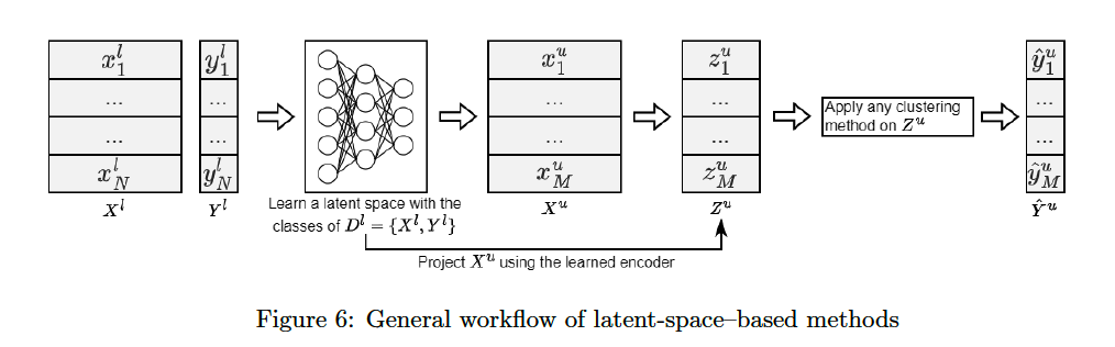
Step 1) Train latent representation with \(D^l=\left\{X^l, Y^l\right\}\)

• incorporates the important characteristics of the known classes \(\mathcal{Y}^l\).

• using DNN classifier ( CE loss )

  ( discard output & softmax layers after training )

  ( use the output of last hidden layer )

  • Assumption ) High-level features of the known classes are shared

Step 2) \(X^u\) is then projected as \(Z^{u}\)

• then apply any clustering method to \(Z\)

[ Deep Transfer Clustering (DTC) ]

Extends to the NCD setting a deep clustering method

• based on an unsupervised deep clustering method ( DEC )

  • does not rely on pairwise pseudo labels

  • maintains a list of class prototypes that represent the cluster centers

    & and assigns instances to the closest prototype.

• How to adapt DEC to the NCD setting ?
• Step 1) Initialize a representation by training a classifier with CE loss on \(D^l\)
• Step 2) Embed \(D^u\)
  • obtained by projecting through the classifier from Step 1)
  • (intuition) classes \(Y^l\) and \(Y^u\) share similar semantic features,
• Step 3) Applies DEC with some improvements
  • clusters are slowly annealed to prevent collapsing
  • further reducing the dimension of the learned representation with PCA leads to an improved performance.

[ Meta Discovery with MAML (MM) ]

Formalizes the assumptions behind NCD & proposes to train a set of expert classifiers to cluster the unlabeled data

• proposes a new method along with theoretical contributions to the field of NCD
• Four conditions
  • (1) Known and novel classes must be disjoint
  • (2) It must be meaningful to separate observations from \(X^l\) and \(X^u\)
  • (3) Good high-level features must exist for \(X^l\) or \(X^u\) and based on these features, it must be easy to separate \(X^l\) or \(X^u\)
  • (4) High0level features are shared by \(X^l\) and \(X^u\).
• These four conditions are worthy of consideration when the NCD problem is addressed for a new dataset.
• Suggest that it is possible to cluster \(D^u\) based on the features learned on \(D^l\).

Propose a two-stage approach

• step 1) Training a number of “expert” classifiers on \(D^l\) with a shared feature extractor.
  • classifiers are constrained to be orthogonal to each other
    • to ensure that they each learn to recognize unique features of the labeled data.
  • The resulting latent space should reveal these high-level features
• step 2) Expert classifiers are then fine-tuned on \(D^u\) with the BCE
  • pseudo labels : based on the similarity of instances in the latent representation learned on \(D^l\).

(2) One-stage methods

a) Introduction

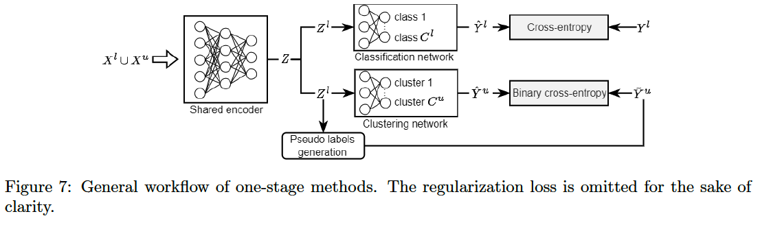
Motivation : Among two-stage approaches, both similarity & latent-space based are negatively impacted when the relevant high-level features are not completely shared by the known and unknown classes

\(\rightarrow\) Exploit both sets \(D^l\) and \(D^u\) simultaneously

By handling both \(D^{l}\) and \(D^{u}\) ….

\(\rightarrow\) One-stage methods will inherently obtain a better latent representation less biased towards the known classes.

For each dataset …

• \(D^l\) : classification ( with labels )
• \(D^u\) : Binarry classification ( with similarity measures )

By training both networks on the same latent space, they share knowledge with other.

Define a multi-objective loss function : 3 components:

• (1) cross entropy \(\left(\mathcal{L}_{C E}\right)\)
• (2) binary cross-entropy \(\left(\mathcal{L}_{B C E}\right)\)
• (3) regularization \(\left(\mathcal{L}_{M S E}\right)\).
  • usually done by encouraging both networks to predict the same class for an instance and its randomly augmented counterpart

b) AutoNovel

( First one-stage method proposed to solve the NCD problem. )

(1) Initializing its encoder using the RotNet

• RotNet : SSL method, predicting rotation
  • trained on both labeled and unlabeled data.
  • does not use labels … no bias towards known classes

(2) Labeled data is used to …

• train for a few epochs the classifier
• fine-tune the last layer of the encoder.

This concludes the initialization of the representation (the shared encoder in Figure 7),

Three components of the model

• (1) shared encoder
• (2) classification network
• (3) clustering network

are then trained using a loss as

\(\mathcal{L}_{\text {AutoNovel }}=\mathcal{L}_{C E}+\mathcal{L}_{B C E}+\mathcal{L}_{M S E}\).

c) Class Discovery Kernel Network with Expansion (CD-KNet-Exp)

Multi-stage method

• constructs a latent representation using \(D^l\) and \(D^u\)

Step 1) Pretraining a representation with a “deep” classifier on \(D^l\) only.

• biased towards the known classes

Step 2) Fine-tune with both \(D^l\) and \(D^u\).

Step 3) Optimize the following objective:

\(\max _{U, \theta} \mathbb{H}\left(f_\theta(X), U\right)+\lambda \mathbb{H}\left(f_\theta\left(X^l\right), Y^l\right)\).

• \(\mathbb{H}(P, Q)\) : Hilbert Schmidt Independence Criterion (HSIC).
  • measures the dependence between distributions \(P\) and \(Q\).
  • \(U\) is the spectral embedding of \(X\).
• First term
  • encourages the separation of all classes by performing something similar to spectral clustering
• Second term
  • maximizing the dependence between the embedding of \(X^l\) and its labels \(Y^l\)

Final Prediction ) \(f_\theta\left(X^u\right)\) partitioned with \(k\)-means clustering.

d) OpenMix

Exploit the labeled data to generate more robust pseudo labels for the unlabeled data

• relies on MixUp
  • requires labeled samples for every class of interest,
  • applying it directly on the unlabeled data would still produce unreliable pseudo labels.
• OpenMix : generates new training samples by mixing both labeled and unlabeled samples.

Step 1) Latent representation is initialized using the \(D^{l}\) only

Step 2) Clustering network is defined to discover the new classes

• using a joint loss on \(D^l\) and \(D^u\).
• trained with synthetic data that are a mix of a sample from \(D^{l}\) & \(D^{u}\)
  • labels : combination of …
    • GT labels of the labeled samples
    • pseudo labels determined using cosine similarity for the unlabeled samples

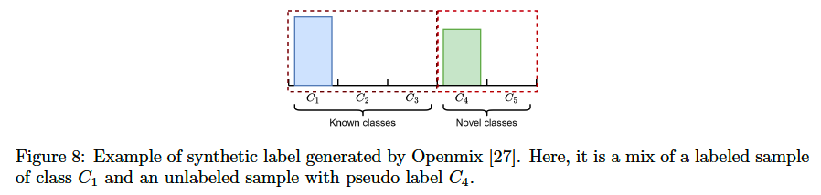
\(\rightarrow\) Overall uncertainty of the resulting pseudo labels will be reduced

( as the labeled counterpart does not belong to any new class and its label distribution is exactly true )

e) Neighborrhood Contrastive Learning (NCL)

• inspired by AutoNovel ( & same architecture (Figure 7) )

• Main contribution

  = Addition of 2 contrastive learning terms

2 CL loss

• (1) Supervised CL

  • applied to the labeled data

• (2) Original unsupervised CL

  • applied on the unlabeled data

  • maintain a queue \(M^u\) of samples from past training steps

    & consider for any instance in a batch that the \(k\) most similar instances from the queue are most likely from the same class.

  • \(l\left(z_i^u, \rho_k\right)=-\frac{1}{k} \sum_{\bar{z}_j^u \in \rho_k} \log \frac{e^{\delta\left(z_i^u, \bar{z}_j^u\right) / \tau}}{e^{\delta\left(z_i^u, \hat{z}_i^u\right) / \tau}+\sum_{m=1}^{ \mid M^u \mid } e^{\delta\left(z_i^u, \bar{z}_m^u\right) / \tau}}\).

    • \(\rho_k\) : \(k\) instances most similar to \(z_i^u\) in the unlabeled queue \(M^u\)
    • \(\delta\) :similarity function
    • \(\tau\) : temperature parameter.

Also, synthetic positive pairs \(\left(z^u, \hat{z}^u\right)\) are generated

• by randomly augmenting each instance.
• The contrastive loss for positive pairs is written as:
  • \(l\left(z^u, \hat{z}^u\right)=-\log \frac{e^{\delta\left(z^u, \hat{z}^u\right) / \tau}}{e^{\delta\left(z^u, \hat{z}^u\right) / \tau}+\sum_{m=1}^{\mid M^u} e^{\delta\left(z^u, \bar{z}_m^u\right) / \tau}}\).

“Hard negatives”

( = similar samples that belong to a different class )

• introduced in the queue \(M^u\) to further improve the learning process.

• Selecting hard negatives in \(D^u\) can be difficult

  ( since there are no class labels )

• Authors take advantage of the fact that the classes of \(D^l\) and \(D^u\) are necessarily disjoint and create new hard negative samples by interpolating

  • (1) easy negatives from the unlabeled set &
  • (2) hard negatives from the labeled se

  
  

Overall loss : \(\mathcal{L}_{N C L}=\mathcal{L}_{\text {AutoNovel }}+l_{s c l}+\alpha l\left(z_i^u, \rho_k\right)+(1-\alpha) l\left(z^u, \hat{z}^u\right)\)

• \(l_{s c l}\) : supervised CL term for \(D^l\)

f) Other Method

pass

(3) Estimating the number of unknown classes

Automatically estimate this number \(C^u\).

Examples) [5, 19, 30, 37]

• set the number of output neurons of the clustering network to a large number (e.g. 100).

• rely on the clustering network to use only the necessary number of clusters

• Clusters are counted if they contain more instances than a certain threshold.

Examples) [12, 38]

• \(k\)-means is performed on \(D^l \cup D^u\).
• The number of unknown classes \(C^u\) is estimated to be the \(k\) that maximized the Hungarian clustering accuracy

Examples ) [14, 18, 13, 39]

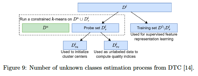
• make use of the known classes
• known classes of \(D^l\) are first split into
  • a probe subset \(D_r^l\)
    • combined with the unlabeled set \(D^u\).
  • a training subset \(D^l \backslash D_r^l\) containing the remaining classes.
    • used for supervised feature representation learning,
• Constrained \(k\)-means is run on \(D_r^l \cup D^u\).
• Part of the classes of \(D_r^l\) are used for the clusters initialization, while the rest are used to compute 2 cluster quality indices (average clustering accuracy and cluster validity index).

(4) Methods Summarry

4. New domains derived from NCD

As the number of NCD works increases, new domains closely related to it are emerging.

• relax some of the hypotheses
• define new tasks inspired by NCD.

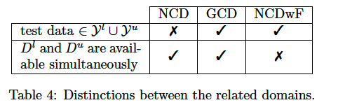
[ Generalized Category Discovery (GCD) ]

[ Novel Clas Discovery without Forgetting (NCDwF) ]

[ Novel Clas Discovery in Semantic Segmentation (NCDSS) ]