(paper 89) Non-autoregressive Conditional Diffusion Models for Time Series Prediction

Non-autoregressive Conditional Diffusion Models for Time Series Prediction

Contents

1. Abstract
2. Introduction
   1. Autoregressive
   2. Non-autoregressive
3. Preliminaries
   1. DDPM
   2. Conditional DDPMs for TS Prediction
   3. TimeGrad
   4. CSDI
   5. SSSD
4. Proposed Model
   1. Forward Diffusion Process
   2. Backward Diffusion Process
   3. Denoising Network
   4. Training

0. Abstract

Denoising diffusion models

• Excel in the generation of images, audio and text.
• Not yet in TS

TimeDiff

• Non-autoregressive diffusion model

• Two novel conditioning mechanisms:

  • (1) Future Mixup

    • similar to teacher forcing

      ( allows parts of the GT future predictions for conditioning )

  • (2) Autoregressive Initialization

    • helps better initialize the model with basic time series patterns such as short-term trends.

• Experiments : 9 real-world datasets.

1. Introduction

Existing TS diffusion models : 2 categories by decoding strategy

• (1) Autoregressive
• (2) Non-autoregressive

(1) Autoregrerssive

• ex) Rasul et al., 2021 & Yang et al., 2022
• future predictions are generated one by one over time.
• limitation in LONG-range prediction performance
  • due to error accumulation & slow inference speed

(2) Non-autoregressive

• ex) CSDI (Tashiro et al., 2021) & SSSD (Alcaraz & Strodthoff, 2022).

• conditioning in the denoising networks’ intermediate layers and introduce inductive bias into the denoising objective.

• long-range prediction performance : worse than Fedformer

  ( \(\because\) conditioning strategies are from image or text data, but not tailored for TS )

• Only using the denoising objective to introduce inductive bias may not be sufficient to guide the conditioning network in capturing helpful information from the lookback window, leading to inaccurate predictions.

TimeDiff

• a Conditional Non-autoregressive Diffusion model for LTSF

• introduces additional inductive bias in the conditioning module that is tailor-made for TS
• Two conditioning mechanisms
  • (i) Future Mixup
    • randomly reveals parts of the ground-truth future predictions during training
  • (ii) Autoregressive Initialization
    • better initializes the model with basic components in TS
• Experimental results on 9 real-world datasets

2. Preliminaries

Diffusion models

• (1) Forward diffusion process
• (2) Backward denoising process.

(1) Denoising Diffusion Probabilistic Model (DDPM)

gradually adding noise

a) Forward diffusion process ( \(K\) steps ) :

transforms \(\mathbf{x}^0\) to a white Gaussian noise vector \(\mathbf{x}^K\)

• \(q\left(\mathbf{x}^k \mid \mathbf{x}^{k-1}\right)=\mathcal{N}\left(\mathbf{x}^k ; \sqrt{1-\beta_k} \mathbf{x}^{k-1}, \beta_k \mathbf{I}\right)\).

  • where \(\beta_k \in[0,1]\) is the noise variance

    ( following a predefined schedule )

\(q\left(\mathbf{x}^k \mid \mathbf{x}^0\right)=\mathcal{N}\left(\mathbf{x}^k ; \sqrt{\bar{\alpha}_k} \mathbf{x}^0,\left(1-\bar{\alpha}_k\right) \mathbf{I}\right)\).

• where \(\alpha_k:=1-\beta_k\) and \(\bar{\alpha}_k:=\Pi_{s=1}^k \alpha_s\).

\(\mathbf{x}^k=\sqrt{\bar{\alpha}_k} \mathbf{x}^0+\sqrt{1-\bar{\alpha}_k} \epsilon,\).

• where \(\epsilon\) is sampled from \(\mathcal{N}(0, \mathbf{I})\).

b) Backward denoising process ( = Markovian process )

\(p_\theta\left(\mathbf{x}^{k-1} \mid \mathbf{x}^k\right)=\mathcal{N}\left(\mathbf{x}^{k-1} ; \mu_\theta\left(\mathbf{x}^k, k\right), \Sigma_\theta\left(\mathbf{x}^k, k\right)\right)\).

• \(\Sigma_\theta\left(\mathbf{x}^k, k\right)\) is often fixed at \(\sigma_k^2 \mathbf{I}\)
• \(\mu_\theta\left(\mathbf{x}^k, k\right)\) is modeled by a NN

c) Training the Diffusion Model

• uniformly samples \(k\) from \(\{1,2, \ldots, K\}\)

• minimizes \(\mathcal{L}_k=D_{\mathrm{KL}}\left(q\left(\mathbf{x}^{k-1} \mid \mathbf{x}^k\right) \| p_\theta\left(\mathbf{x}^{k-1} \mid \mathbf{x}^k\right)\right)\).

  ( = learning the denoising process )

For more stable training, \(q\left(\mathbf{x}^{k-1} \mid \mathbf{x}^k\right)\) is often replaced by

\(q\left(\mathbf{x}^{k-1} \mid \mathbf{x}^k, \mathbf{x}^0\right)=\mathcal{N}\left(\mathbf{x}^{k-1} ; \tilde{\mu}_k\left(\mathbf{x}^k, \mathbf{x}^0, k\right), \tilde{\beta}_k \mathbf{I}\right)\).

• \(\tilde{\mu}_k\left(\mathbf{x}^k, \mathbf{x}^0, k\right)=\frac{\sqrt{\bar{\alpha}_{k-1}} \beta_k}{1-\bar{\alpha}_k} \mathbf{x}^0+\frac{\sqrt{\alpha_k}\left(1-\bar{\alpha}_{k-1}\right)}{1-\bar{\alpha}_k} \mathbf{x}^k\).
• \(\tilde{\beta}_k=\frac{1-\bar{\alpha}_{k-1}}{1-\bar{\alpha}_k} \beta_k\).

d) Training Objective

Rewritten as…

\(\mathcal{L}_k=\frac{1}{2 \sigma_k^2}\left\|\tilde{\mu}_k\left(\mathbf{x}^k, \mathbf{x}^0, k\right)-\mu_\theta\left(\mathbf{x}^k, k\right)\right\|^2\).

( = ignoring the variance term )

\(\mu_\theta\left(\mathbf{x}^k, k\right)\) can be defined in 2ways

• (1) \(\mu_\epsilon\left(\epsilon_\theta\right)\) : from NOISE prediction model
• (2) \(\mu_{\mathbf{x}}\left(\mathbf{x}_\theta\right)\) : from DATA prediction model

(1) \(\mu_\epsilon\left(\epsilon_\theta\right)=\frac{1}{\sqrt{\alpha_k}} \mathbf{x}^k-\frac{1-\alpha_k}{\sqrt{1-\bar{\alpha}_k} \sqrt{\alpha_k}} \epsilon_\theta\left(\mathbf{x}^k, k\right)\).

• computed from a noise prediction model \(\epsilon_\theta\left(\mathbf{x}^k, k\right)\)

• optimizing the following simplified training objective leads to better generation quality ( Ho et al. (2020) )

  \(\mathcal{L}_\epsilon=\mathbb{E}_{k, \mathbf{x}^0, \epsilon}\left[\left\|\epsilon-\epsilon_\theta\left(\mathbf{x}^k, k\right)\right\|^2\right]\).

  • \(\epsilon\) : noise used to obtain \(\mathbf{x}^k\) from \(\mathbf{x}^0\) at step \(k\)

(2) \(\mu_{\mathbf{x}}\left(\mathbf{x}_\theta\right)=\frac{\sqrt{\alpha_k}\left(1-\bar{\alpha}_{k-1}\right)}{1-\bar{\alpha}_k} \mathbf{x}^k+\frac{\sqrt{\bar{\alpha}_{k-1}} \beta_k}{1-\bar{\alpha}_k} \mathbf{x}_\theta\left(\mathbf{x}^k, k\right)\).

• from a data prediction model \(\mathbf{x}_\theta\left(\mathbf{x}^k, k\right)\)
• \(\mathcal{L}_{\mathbf{x}}=\mathbb{E}_{k, \mathbf{x}^0, \epsilon}\left[\left\|\mathbf{x}^0-\mathbf{x}_\theta\left(\mathbf{x}^k, k\right)\right\|^2\right]\).

\(\rightarrow\) both (1) & (2) : conditioned on the diffusion step \(k\) only.

• When an additional condition input \(\mathbf{c}\) is available, can be injected

  \(p_\theta\left(\mathbf{x}^{k-1} \mid \mathbf{x}^k, \mathbf{c}\right)=\mathcal{N}\left(\mathbf{x}^{k-1} ; \mu_\theta\left(\mathbf{x}^k, k \mid \mathbf{c}\right), \sigma_k^2 \mathbf{I}\right)\).

  \(\mu_{\mathbf{x}}\left(\mathbf{x}_\theta\right)=\frac{\sqrt{\alpha_k}\left(1-\bar{\alpha}_{k-1}\right)}{1-\bar{\alpha}_k} \mathbf{x}^k+\frac{\sqrt{\bar{\alpha}_{k-1}} \beta_k}{1-\bar{\alpha}_k} \mathbf{x}_\theta\left(\mathbf{x}^k, k \mid \mathbf{c}\right)\).

(2) Conditional DDPMs for TS Prediction

Notation

• Input : \(\mathbf{x}_{-L+1: 0}^0 \in \mathbb{R}^{d \times L}\)

• Target : \(\mathbf{x}_{1: H}^0 \in \mathbb{R}^{d \times H}\)

Conditional DDPMs

• \(p_\theta\left(\mathrm{x}_{1: H}^{0: K} \mid \mathbf{c}\right)=p_\theta\left(\mathrm{x}_{1: H}^K\right) \prod_{k=1}^K p_\theta\left(\mathrm{x}_{1: H}^{k-1} \mid \mathrm{x}_{1: H}^k, \mathbf{c}\right)\).
  • \[\mathbf{x}_{1: H}^K \sim \mathcal{N}(\mathbf{0}, \mathbf{I})\]
  • \(\mathbf{c}=\mathcal{F}\left(\mathbf{x}_{-L+1: 0}^0\right)\) is the output of the conditioning network \(\mathcal{F}\)
• \(p_\theta\left(\mathbf{x}_{1: H}^{k-1} \mid \mathbf{x}_{1: H}^k, \mathbf{c}\right)=\mathcal{N}\left(\mathbf{x}_{1: H}^{k-1} ; \mu_\theta\left(\mathbf{x}_{1: H}^k, k \mid \mathbf{c}\right), \sigma_k^2 \mathbf{I}\right)\).

(3) TimeGrad (Rasul et al., 2021)

Denoising diffusion model for TS prediction

• autoregressive model
• model the joint distribution \(p_\theta\left(\mathbf{x}_{1: H}^{0: K}\right)\),
  • where \(\mathbf{x}_{1: H}^{0: K}=\left\{\mathbf{x}_{1: H}^0\right\} \bigcup\left\{\mathbf{x}_{1: H}^k\right\}_{k=1, \ldots, K}\)

\(\begin{aligned} p_\theta & \left(\mathbf{x}_{1: H}^{0: K} \mid \mathbf{c}=\mathcal{F}\left(\mathbf{x}_{-L+1: 0}^0\right)\right) \\ & =\prod_{t=1}^H p_\theta\left(\mathbf{x}_t^{0: K} \mid \mathbf{c}=\mathcal{F}\left(\mathbf{x}_{-L+1: t-1}^0\right)\right) \\ & =\prod_{t=1}^H p_\theta\left(\mathbf{x}_t^K\right) \prod_{k=1}^K p_\theta\left(\mathbf{x}_t^{k-1} \mid \mathbf{x}_t^k, \mathbf{c}=\mathcal{F}\left(\mathbf{x}_{-L+1: t-1}^0\right)\right) \end{aligned}\).

\(\mathcal{F}\) : RNN

• uses its hidden state \(\mathbf{h}_t\) as \(c\)

Objective function :

• \(\mathcal{L}_\epsilon=\mathbb{E}_{k, \mathbf{x}^0, \epsilon}\left[\left\|\epsilon-\epsilon_\theta\left(\mathbf{x}_t^k, k \mid \mathbf{h}_t\right)\right\|^2\right]\).

Pros & Cons

• Pros ) Successfully used for short-term TS prediction

• Conse ) Due to autoregressive decoding

  \(\rightarrow\) error can accumulate and inference is also slow.

  BAD for long-term TS prediction

(4) CSDI (Tashiro et al., 2021)

Non-autoregressive inference

• by diffusing and denoising the whole time series \(\mathbf{x}_{-L+1: H}^0\).

Two Inputs of denoising model

• (1) \(\mathbf{x}_{-L+1: H}^0\)
• (2) Binary mask \(\mathbf{m} \in\{0,1\}^{d \times(L+H)}\)
  • where \(\mathbf{m}_{i, t}=0\) if position \(i\) is observed at time \(t\), and 1 otherwise.

SSL strategy : masking some input observations

• \(\mathcal{L}_\epsilon=\mathbb{E}_{k, \mathbf{x}^0, \epsilon}\left[\left\|\epsilon-\epsilon_\theta\left(\mathbf{x}_{\text {target }}^k, k \mid \mathbf{c}=\mathcal{F}\left(\mathbf{x}_{\text {observed }}^k\right)\right)\right\|^2\right]\).
  • \(\mathbf{x}_{\text {target }}^k=\mathbf{m} \odot \mathbf{x}_{-L+1: H}^0\) : the masked part
  • \(\mathbf{x}_{\text {observed }}^k=(1-\mathbf{m}) \odot \mathbf{x}_{-L+1: H}^0\) : the observed part.

CSDI is still limited in 2 aspects:

• (1) CSDI’s denoising network is based on 2 transformers,
  • complexity issue
• (ii) Its conditioning is based on masking,
  • may cause disharmony at the boundaries between masked & observed regions

(5) SSSD (Alcaraz \& Strodthoff, 2022)

replaces transformers \(\rightarrow\) structured state space model

• Avoids the quadratic complexity issue.

Non-autoregressive strategy

• still have deteriorated performance due to boundary disharmony.

Others

NLP : develop sequence diffusion models with nonautoregressive decoding over time

• e.g., DiffuSeq (Gong et al., 2023).

TS prediction : more challenging …

• as this requires modeling temporal dependencies on irregular, highly nonlinear, and noisy data.

3. Proposed Model

Conditional Diffusion models : widely used

• usually focus on capturing the semantic similarities across modalities (e.g., text and image) (Choi et al., 2021; Kim et al., 2022).

• HOWEVER, in non-stationary TS

  \(\rightarrow\) capturing the complex temporal dependencies maybe even more important.

Propose TimeDiff

• novel conditioning mechanisms that are tailored for TS

(1) Forward Diffusion Process

Diffusion on forecast window

\(\mathbf{x}_{1: H}^k=\sqrt{\bar{\alpha}_k} \mathbf{x}_{1: H}^0+\sqrt{1-\bar{\alpha}_k} \epsilon,\).

• \(\epsilon\) : sampled from \(\mathcal{N}(0, \mathbf{I})\)

• \(D^3 \mathrm{VAE}\) : same forward diffusion process on the lookback window

  • NOT a diffusion model as the diffused \(\mathbf{x}_{1: H}^k\) is produced by a VAE
    • with \(\mathbf{x}_{-L+1: 0}^k\) (instead of \(\mathbf{x}_{1: H}^k\) ) as input
    • does not denoise from random noise.

(2) Backward Denoising Process

\(k\) th denoising step )

• \(\mathbf{x}_{1: H}^k\) is denoised to \(\mathbf{x}_{1: H}^{k-1}\).

To well predict the future TS segment \(\mathbf{x}_{1: H}^0\) …

• useful information needs to be extracted from the lookback window \(\mathbf{x}_{-L+1: 0}^0\)

\(\rightarrow\) to guide the denoising of \(\mathbf{x}_{1: H}^k\) to \(\mathbf{x}_{1: H}^0\)

Proposed inductive bias on the conditioning network : specific to TS prediction.

Section Intro

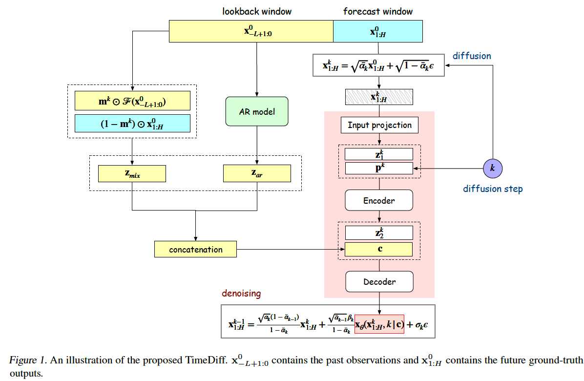
• 3.2.1) Mixup : to combine the past & future TS information into \(\mathbf{z}_{\operatorname{mix}}\)
• 3.2.2) AR model to produce a crude approximation \(\mathbf{z}_{a r}\) of \(\mathbf{x}_{1: H}^0\).

\(\rightarrow\) These two are concatenated & become condition

• \(\mathbf{c}=\operatorname{concat}\left(\left[\mathbf{z}_{\mathrm{mix}}, \mathbf{z}_{a r}\right]\right) \in \mathbb{R}^{2 d \times H}\).

a) Future Mixup ( condition 1 : \(\mathbf{z}_{\text {mix }}\) )

Goal : predict \(\mathbf{x}_{1: H}^0\),

Ideal condition to guide denosing process : \(\mathbf{x}_{1: H}^0\)

• cannot be accessed on inference, but available during training

Future mixup : combines

• (1) the PAST information’s mapping \(\mathcal{F}\left(\mathbf{x}_{-L+1: 0}^0\right)\)
• (2) the FUTURE ground-truth \(\mathbf{x}_{1: H}^0\).

Conditioning signal ( at diffusion step \(k\) )

• \(\mathbf{z}_{\text {mix }}=\mathbf{m}^k \odot \mathcal{F}\left(\mathbf{x}_{-L+1: 0}^0\right)+\left(1-\mathbf{m}^k\right) \odot \mathbf{x}_{1: H}^0\).
  • \(\mathbf{m}^k \in[0,1)^{d \times H}\) : mixing matrix ( from uniform distn )
  • \(\mathcal{F}\) : CNN

But \(\mathbf{x}_{1: H}^0\) is no longer available on inference!

Thus, use below instead.

• \(\mathbf{z}_{\operatorname{mix}}=\mathcal{F}\left(\mathbf{x}_{-L+1: 0}^0\right)\).

Similar to Teacher Forcing & Scheduled Sampling

• (training) introduce GT as during training
• (inference) use model’s prediction during inference.

Difference :

• Future mixup :
  • for non-autoregressive conditional generation in TS diffusion models,
  • mixes the past observations’ embedding and future TS
• Teacher forcing & Scheduled sampling :
  • for autoregressive decoding of RNN
  • replace the model’s prediction at the previous step by the past GT

b) AR model ( condition 2 : \(\mathbf{z}_{\text {ar}}\) )

( Image Impainiting )

• Non-autoregressive models : produce disharmony at the boundaries between masked and observed regions

( TS Prediction )

• disharmony between the history and forecast segment

Linear AR model \(\mathcal{M}_{a r}\)

• to provide an initial guess \(\mathbf{z}_{a r} \in \mathbb{R}^{d \times H}\) for \(\mathbf{x}_{1: H}^0\).

\(\mathbf{z}_{a r}=\sum_{i=-L+1}^0 \mathbf{W}_i \odot \mathbf{X}_i^0+\mathbf{B}\).

• \(\mathbf{x}_i^0\) : the \(i\) th column of \(\mathbf{x}_{-L+1: 0}^0\).
• \(\mathbf{X}_i^0 \in \mathbb{R}^{d \times H}\) : a matrix containing \(H\) copies of \(\mathbf{x}_i^0\)
• \(\mathbf{W}_i\) ‘s \(\in \mathbb{R}^{d \times H}, \mathbf{B} \in \mathbb{R}^{d \times H}\)

Pretrained on the training set …

• by minimizing the \(\ell_2\)-distance between \(\mathbf{z}_{a r}\) and the GT \(\mathrm{x}_{1: H}^0\).

This simple AR model cannot accurately approximate a complex nonlinear TS

But still capture simple patterns, such as short-term trends

Although \(\mathcal{M}_{a r}\) is an AR model, does not require AR decoding.

( = all columns of \(\mathbf{z}_{a r}\) are obtained simultaneously )

(3) Denoising Network

How to denoise \(\mathbf{x}_{1: H}^k \in \mathbb{R}^{d \times H}\) ?

[ Procedure ]

step 1) combine (a) & (b) ( along the channel dimension )

• (a) Diffusion-step embedding : \(\mathbf{p}^k\)
  • obtained using the transformer’s sinusoidal position embedding
  • \(\mathbf{p}^k=\operatorname{SiLU}\left(\mathrm{FC}\left(\operatorname{SiLU}\left(\mathrm{FC}\left(k_{\text {embedding }}\right)\right)\right)\right) \in \mathbb{R}^{d^{\prime} \times 1}\).
  • ( For the concatenation ) broadcasted over length to form \(\left[\mathbf{p}^k, \ldots, \mathbf{p}^k\right] \in \mathbb{R}^{d^{\prime} \times H}\),
• (b) Diffused input \(\mathrm{x}_{1: H}^k\) ‘s embedding : \(\mathbf{z}_1^k \in \mathbb{R}^{d^{\prime} \times H}\)
  • obtained by an input projection block consisting of several CNN layers
• result : Tensor of size \(2 d^{\prime} \times H\).

step 2) Encoding

• encoder : using Multi-layer CNN encoder

• result : representation \(\mathbf{z}_2^k \in \mathbb{R}^{d^{\prime \prime} \times H}\).

step 3) Concatenate \(\mathbf{c}\) and \(\mathbf{z}_2^k\).

• result : input of size \(\left(2 d+d^{\prime \prime}\right) \times H\). ( to decoder )

Step 4) Decoding

• decoder : using Multi-layer CNN encoder
• result : \(\mathbf{x}_\theta\left(\mathbf{x}_{1: H}^k, k \mid \mathbf{c}\right)\) …. of size \(d \times H\) ( = the same as \(\mathbf{x}_{1: H}^k\). )

Step 5) Denoised output \(\hat{\mathbf{x}}_{1: H}^{k-1}\)

• \(\hat{\mathbf{x}}_{1: H}^{k-1}= \frac{\sqrt{\alpha_k}\left(1-\bar{\alpha}_{k-1}\right)}{1-\bar{\alpha}_k} \mathbf{x}_{1: H}^k+\frac{\sqrt{\bar{\alpha}_{k-1}} \beta_k}{1-\bar{\alpha}_k} \mathbf{x}_\theta\left(\mathbf{x}_{1: H}^k, k \mid \mathbf{c}\right) +\sigma_k \epsilon\).
  • where \(\epsilon \sim \mathcal{N}(\mathbf{0}, \mathbf{I})\).

Note that we predict the data \(\mathbf{x}_\theta\left(\mathbf{x}_{1: H}^k, k\right)\) for denoising,

( rather than predicting the noise \(\epsilon_\theta\left(\mathbf{x}_{1: H}^k, k\right)\) )

As TS usually contain highly irregular noisy components,

\(\rightarrow\) estimating the diffusion noise \(\epsilon\) can be more difficult!

(4) Training

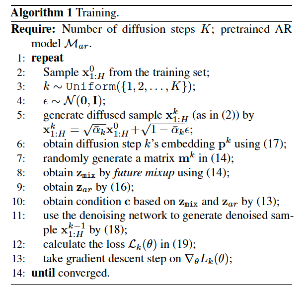
For each \(\mathrm{x}_{1: H}^0\), randomly sample a batch of diffusion steps \(k\) ‘s

Minimize below

\(\min _\theta \mathcal{L}(\theta)=\min _\theta \mathbb{E}_{\mathbf{x}_{1: H}^0, \epsilon \sim \mathcal{N}(\mathbf{0}, \mathbf{I}), k} \mathcal{L}_k(\theta)\),

• \(\mathcal{L}_k(\theta)=\left\|\mathbf{x}_{1: H}^0-\mathbf{x}_\theta\left(\mathbf{x}_{1: H}^k, k \mid \mathbf{c}\right)\right\|^2\).

(5) Inference

Generate a noise vector \(\mathbf{x}_{1: H}^K \sim \mathcal{N}(\mathbf{0}, \mathbf{I})\)

• size \(d \times H\).

Repeatedly run the denoising step ( until \(k=1\) )

Obtain the time series \(\hat{\mathbf{x}}_{1: H}^0\) as final prediction.