(paper) Time-series Generative Adversarial Networks

Time-series Generative Adversarial Networks (2019)

Contents

1. Abstract
2. Introduction
3. Dilated RNN
   1. Dilated recurrent skip-connection
   2. Exponentially Increasing Dilation

0. Abstract

기존에 존재하는 sequential setting 하에서의 GAN은, temporal correlation 제대로 고려 X

따라서, propose a novel framework for generating realistic time-series..

• that combines “the flexibility of UNSUPERVISED paradigm”
• with the “control afforded by SUPERVISED training”

1. Introduction

when modeling multivariate sequential data \(\mathrm{x}_{1: T}=\left(\mathrm{x}_{1}, \ldots, \mathrm{x}_{T}\right)\),

• wish to capture conditional distribution \(p\left(\mathrm{x}_{t} \mid \mathrm{x}_{1: t-1}\right)\) of temporal transitions

Autoregressive models

• factor the distribution of sequences into \(\prod_{t} p\left(\mathrm{x}_{t} \mid \mathrm{x}_{1: t-1}\right)\)

• deterministic, not generative in that

  new sequences can be randomly sampled from them, without external conditioning

GAN

• instantiating RNN for the role of G & D
• but, do not leverage the autoregressive prior
• simply summing the standard GAN loss may not be sufficient!

This paper, Autoregressive Model + GAN \(\rightarrow\) TimeGAN

• 1) introduce stepwise supervised loss, using the original data as supervision
• 2) introduce embedding network to provide reversible mapping between \(X\) & \(Z\)
• 3) generalize this framework to handle mixed-data setting

2. Problem Formulation

Notation

• \(\mathcal{S}\) : vector space of static features

• \(\mathcal{X}\) : vector space of temporal features

  \(\rightarrow\) consider tuples of the form \(\left(\mathbf{S}, \mathbf{X}_{1: T}\right)\) with some joint distribution \(p\).

  ( length \(T\) is also random variable )

• training data : \(\mathcal{D}=\left\{\left(\mathbf{s}_{n}, \mathbf{x}_{n, 1: T_{n}}\right)\right\}_{n=1}^{N} .\)

Goal

• use \(\mathcal{D}\) to learn \(\hat{p}\left(\mathbf{S}, \mathbf{X}_{1: T}\right)\) that best approximates \(p\left(\mathbf{S}, \mathbf{X}_{1: T}\right)\)
• make use of autoregressive decomposition : \(p\left(\mathbf{S}, \mathbf{X}_{1: T}\right)=p(\mathbf{S}) \prod_{t} p\left(\mathbf{X}_{t} \mid \mathbf{S}, \mathbf{X}_{1: t-1}\right)\)

Two Objectives

(1) Global

• \(\min _{\hat{p}} D\left(p\left(\mathbf{S}, \mathbf{X}_{1: T}\right) \mid \mid \hat{p}\left(\mathbf{S}, \mathbf{X}_{1: T}\right)\right)\).
• Jensen-Shannon divergence
• relies on the presence of perfect adversary ( have no access to )

(2) Local

• \(\min _{\hat{p}} D\left(p\left(\mathbf{X}_{t} \mid \mathbf{S}, \mathbf{X}_{1: t-1}\right) \mid \mid \hat{p}\left(\mathbf{X}_{t} \mid \mathbf{S}, \mathbf{X}_{1: t-1}\right)\right)\). for any \(t\)
• only depends on the presence of ground-truth sequence ( have access to )

(3) Summary

• combination of GAN objective ( proportional to (1) ) & ML objective ( proportional to (2) )

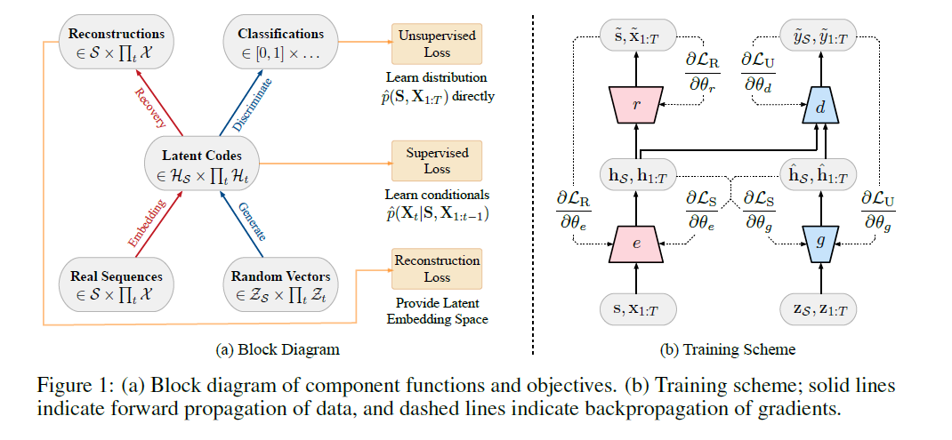
3. Proposed Model : TimeGAN

TimeGAN = 4 components

[ Auto-encoding components]

• 1) embedding function
• 2) recovery function
  

[ Adversarial components ]

• 3) sequence generator
• 4) sequence discriminator

TimeGAN simulatneously learns to..

• 1) encode features
• 2) generate representations
• 3) iterate across time

3-1) Embedding Function & Recovery Function

Two functions :

• provide mapping between “feature” & “latent space”
• allow adversarial network to learn in LOWER-dimension

Notation

• \(\mathcal{H}_{\mathcal{S}}, \mathcal{H}_{\mathcal{X}}\) : latent vector spaces corresponding to feature spaces \(\mathcal{S}, \mathcal{X}\)

[1] Embedding Function

• \(e: \mathcal{S} \times \prod_{t} \mathcal{X} \rightarrow \mathcal{H}_{\mathcal{S}} \times \prod_{t} \mathcal{H}_{\mathcal{X}}\).

• input : static & temporal features

• output : latent codes

  \(\mathbf{h}_{\mathcal{S}}, \mathbf{h}_{1: T}=e\left(\mathbf{s}, \mathbf{x}_{1: T}\right)\).

  • \(\mathbf{h}_{\mathcal{S}}=e_{\mathcal{S}}(\mathbf{s})\).
  • \(\mathbf{h}_{t}=e_{\mathcal{X}}\left(\mathbf{h}_{\mathcal{S}}, \mathbf{h}_{t-1}, \mathbf{x}_{t}\right)\).

[2] Recovery Function

• \(r: \mathcal{H}_{\mathcal{S}} \times \prod_{t} \mathcal{H}_{\mathcal{X}} \rightarrow \mathcal{S} \times \prod_{t} \mathcal{X}\).

• input : latent codes

• output : static & temporal features

  \(\tilde{\mathbf{s}}, \tilde{\mathbf{x}}_{1: T}=r\left(\mathbf{h}_{\mathcal{S}}, \mathbf{h}_{1: T}\right)\).

  • \(\tilde{\mathbf{s}}=r_{\mathcal{S}}\left(\mathbf{h}_{s}\right)\).
  • \(\tilde{\mathbf{x}}_{t}=r_{\mathcal{X}}\left(\mathbf{h}_{t}\right)\).

3-2) Sequence Generator & Sequence Discriminator

[1] Sequence Generator

• Instead of producing synthetic output directly in feature space(X),

  the generator first outputs into the embedding space(O).

• generating function : \(g: \mathcal{Z}_{\mathcal{S}} \times \prod_{t} \mathcal{Z}_{\mathcal{X}} \rightarrow \mathcal{H}_{\mathcal{S}} \times \prod_{t} \mathcal{H}_{\mathcal{X}}\)

  • input : tuple of static & temporal random vectors
  • output : \(\hat{\mathbf{h}}_{\mathcal{S}}, \hat{\mathbf{h}}_{1: T}=g\left(\mathbf{z}_{\mathcal{S}}, \mathbf{z}_{1: T}\right)\).
    • \(\hat{\mathbf{h}}_{\mathcal{S}}=g_{\mathcal{S}}\left(\mathbf{z}_{\mathcal{S}}\right)\).
    • \(\hat{\mathbf{h}}_{t}=g_{\mathcal{X}}\left(\hat{\mathbf{h}}_{\mathcal{S}}, \hat{\mathbf{h}}_{t-1}, \mathbf{z}_{t}\right)\).
  • random vector \(\mathrm{z}_{\mathcal{S}}\) can be sampled from a distribution of choice
  • \(\mathrm{z}_{t}\) follows a stochastic process

[2] Sequence Discriminator

• also operates from the embedding space

• discrimination function : \(d: \mathcal{H}_{\mathcal{S}} \times \prod_{t} \mathcal{H}_{\mathcal{X}} \rightarrow[0,1] \times \prod_{t}[0,1]\)

  • input : static and temporal codes
  • output : classifications \(\tilde{y}_{\mathcal{S}}, \tilde{y}_{1: T}=d\left(\tilde{\mathbf{h}}_{\mathcal{S}}, \tilde{\mathbf{h}}_{1: T}\right)\)

• notation :

  • \(\tilde{\mathbf{h}}_{*}\) : either real \(\left(\mathbf{h}_{*}\right)\) or synthetic \(\left(\hat{\mathbf{h}}_{*}\right)\)embeddings
  • \(\tilde{y}_{*}\) : classifications of either real \(\left(y_{*}\right)\) or synthetic \(\left(\hat{y}_{*}\right)\) data

• implement \(d\) with bidirectional recurrent network with feed forward NN

  • \(\tilde{y}_{\mathcal{S}}=d_{\mathcal{S}}\left(\tilde{\mathbf{h}}_{\mathcal{S}}\right)\).

  • \(\tilde{y}_{t}=d_{\mathcal{X}}\left(\overleftarrow{\mathbf{u}}_{t}, \overrightarrow{\mathbf{u}}_{t}\right)\).

    where

    • \(\overrightarrow{\mathbf{u}}_{t}=\vec{c}_{\mathcal{X}}\left(\tilde{\mathbf{h}}_{\mathcal{S}}, \tilde{\mathbf{h}}_{t}, \overrightarrow{\mathbf{u}}_{t-1}\right)\).
    • \(\stackrel{\leftarrow}{\mathbf{u}}_{t}=\overleftarrow{c}_{\mathcal{X}}\left(\tilde{\mathbf{h}}_{\mathcal{S}}, \tilde{\mathbf{h}}_{t}, \overleftarrow{\mathbf{u}}_{t+1}\right)\).

(3) Jointly Learning to Encode, Generate, Iterate

embedding & recovery function should enable accurate reconstruction \(\tilde{\mathbf{s}}, \tilde{\mathbf{x}}_{1: T}\) of original \(\mathbf{s}, \mathrm{x}_{1: T}\) ,

from their latent representation \(\mathbf{h}_{\mathcal{S}}, \mathbf{h}_{1: T}\)

\(\rightarrow\) 1st objective : RECONSTRUCTION loss

\(\mathcal{L}_{\mathrm{R}}=\mathbb{E}_{\mathbf{s}, \mathbf{x}_{1: T} \sim p}\left[ \mid \mid \mathrm{~s}-\tilde{\mathbf{s}} \mid \mid _{2}+\sum_{t} \mid \mid \mathrm{x}_{t}-\tilde{\mathrm{x}}_{t} \mid \mid _{2}\right]\).

[ Inputs of generator # 1 ]

• synthetic embeddings \(\hat{\mathbf{h}}_{\mathcal{S}}, \hat{\mathbf{h}}_{1: t-1}\) to generate the next synthetic vector \(\hat{\mathbf{h}}_{t}\).
  • gradients are then computed on the “unsupervised loss”
• \(\mathcal{L}_{\mathrm{U}}=\mathbb{E}_{\mathbf{s}, \mathbf{x}_{1: T} \sim p}\left[\log y_{\mathcal{S}}+\sum_{t} \log y_{t}\right]+\mathbb{E}_{\mathbf{s}, \mathbf{x}_{1: T} \sim \hat{p}}\left[\log \left(1-\hat{y}_{\mathcal{S}}\right)+\sum_{t} \log \left(1-\hat{y}_{t}\right)\right]\).

[ Inputs of generator # 2 ]

• receives sequences of embeddings of actual data \(\mathbf{h}_{1: t-1}\) to generate the next latent vector.

  • gradients are then computed on the “supervised loss”

  • captures the discrepancy between \(p\left(\mathbf{H}_{t} \mid \mathbf{H}_{\mathcal{S}}, \mathbf{H}_{1: t-1}\right)\) & \(\hat{p}\left(\mathbf{H}_{t} \mid \mathbf{H}_{\mathcal{S}}, \mathbf{H}_{1: t-1}\right)\)

• \(\mathcal{L}_{\mathrm{S}}=\mathbb{E}_{\mathbf{s}, \mathbf{x}_{1: T} \sim p}\left[\sum_{t} \mid \mid \mathbf{h}_{t}-g_{\mathcal{X}}\left(\mathbf{h}_{\mathcal{S}}, \mathbf{h}_{t-1}, \mathbf{z}_{t}\right) \mid \mid _{2}\right]\).

  • where \(g_{\mathcal{X}}\left(\mathbf{h}_{\mathcal{S}}, \mathbf{h}_{t-1}, \mathbf{z}_{t}\right)\) approximates \(\mathbb{E}_{\mathbf{Z}_{t} \sim \mathcal{N}}\left[\hat{p}\left(\mathbf{H}_{t} \mid \mathbf{H}_{\mathcal{S}}, \mathbf{H}_{1: t-1}, \mathbf{z}_{t}\right)\right]\).

4. Summary