
Multi-step Forecasting via Multi-task Learning (2019)
Contents
- Abstract
- Introduction
- Related Works
- Recursive strategy
- Direct strategy
- Joint strategy
- Multi-task learning
- Auto Encoder Convolutional Recurrent Neural Network
- Method
- Multi-step forecasting strategies
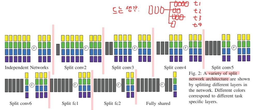
- Split Networks for MTS
- Auxiliary task weights
- Exponential Weighting
0. Abstract
Multi-task learning = improving the GENERALIZATION of a model
제안한 알고리즘의 특징
-
1) enumerating multiple CNN 구조
\(\rightarrow\) balance shared & non-shared layers
-
2) multi-step strategies minimize forecast errors
\(\rightarrow\) loss function들은 서로 다른 scale ( 가까운 미래 vs 멀리 있는 미래 )
1. Introduction
3 main approaches for generating multi-step predictions
- 1) recursive
- 2) direct
- 3) joint
Multi-task learning
- sharing knowledge between different tasks
- set of task is learned in parallel
Multi-task learning에 대한 또 다른 관점
- 1) main task + 2) auxiliary task
Use multi-task learning for MTS (Multivariate Time Series)
- 1) task 자체가 서로 correlated
- 2) internal representation for different tasks 또한 correlated
multi-task 관점의 MTS
- 1) main task = 예측하고자 하는 future points
- 2) auxiliary task = 예측 하고자하는 것 외의 시간 points
여기서 드는 의문점들
- Q 1) 얼마나 share하고, 얼마나 task-specific 해야하나?
- Q 2) main task에 보다 bias 되도록 모델링을 하는 방법은?
- Q 3) 가까운 미래 vs 먼 미래의 uncertainty 차이 반영은?
의문점에 대한 해답
- A 1) search for optimal combination ( via CNN )
- A 2) & A 3) by adopting task weights
제안한 것들
-
factorization of weight vector for the learning task based on the categorization of tasks into main / auxiliary tasks
\(\rightarrow\) search for only 2 params
Contribution
(1) train variety of Split network \(\rightarrow\) right balance between common & task-specific
(2) propose novel multi-task loss
(3) demonstrate the importance of loss weights for number of tasks
2. Related Works
2-1) Recursive strategy
- SVR (Support Vector Machine Regression), RNNs, LSTMs
- LSTM based encoder-decoder architecture
2-2) Direct strategy
- multivariate ARIMA
- NN & KNN
\(\rightarrow\) 2-1) & 2-2) 중 어느 하나가 더 낫다고 단정 X
( 둘 다 공통 단점 : SINGLE output )
2-3) Joint strategy
- 2-3) > 2-1) & 2-2)
- NN can deal with MULTIPLE outputs
2-4) Multi-task learning
2 design choices
- 1) hard-parameter sharing
- sharing all hidden layers
- except final layers
- 2) soft-parameter sharing
- own model & parameters
- use regularization to incorporate multi-task learning
- ex) Split Network
- instead of regularization
- split into shared & non-shared layers
2-5) Auto Encoder Convolutional Recurrent Neural Network
-
problem formulation w.r.t a target time series like ours
-
Algorithm
- step 1) learns filters ( across separate time series )
- step 2) apply pooling to each series output
- step 3) merge them
- step 4) feed them to RNN prediction ( multi-step prediction )
-
이 논문에서 제안한 방법의 차이점은?
-
by SHARED representation between convolutional layers!
-
(이전) uniform weight
(제안) novel multi-task loss ( task 따라 weight 다르게 )
- main & auxiliary series target 따라!
-
3. Method
multi-variate & multi-step
Notation
- future values of \(N\) time series : \(Y=\left\{Y_{1}, Y_{2}, \ldots, Y_{N}\right\}\)
- past input : \(X=\left\{X_{1}, X_{2}, . ., X_{N}\right\}\)
- each time series is MULTIVARIATE ( with \(K\) channels )
- \(Y_{i}=Y_{i}^{*}, Y_{i}^{1}, Y_{i}^{2}, \ldots Y_{i}^{K-1}\).
- \(X_{i}=X_{i}^{*}, X_{i}^{1}, X_{i}^{2}, \ldots, X_{i}^{K-1}\).
- 별표 붙은 애들 = target time series
- \(Y_{i}^{*}=\left\{y_{i, t=h+1}^{*}, y_{i, t=h+2}^{*}, . ., y_{i, t=H}^{*}\right\}\).
- \(h\) : maximum # of time steps for input
- \(X_{i}^{*}=\left\{x_{i, t=0}^{*}, x_{i, t=1}^{*}, . ., x_{i, t=h}^{*}\right\}\).
- \(H\) : maximum # of time steps for output
- \(Y_{i}^{*}=\left\{y_{i, t=h+1}^{*}, y_{i, t=h+2}^{*}, . ., y_{i, t=H}^{*}\right\}\).
- 별표 안 붙은 애들 = auxiliary time series
- 별표 붙은 애들 = target time series
3-1) Multi-step forecasting strategies
multi-step prediction of target series \(Y_{i}^{*}=\left\{y_{i, t=h+1}^{*}, y_{i, t=h+2}^{*}, . ., y_{i, t=H}^{*}\right\}\)
[1] Iterative strategy
- single step prediction
- (one step) \(Y_{t=h+1}^{*}=f\left(X^{*}\right)\).
- (two step) \(Y_{t=h+2}^{*}=f\left(X^{*} \cup Y_{t=h+1}^{*}\right)\)
[2] Direct strategy
- multiple independent models
- (one step) \(Y_{t=h+1}^{*}=f\left(X^{*}\right)\).
- (two step) \(Y_{t=h+2}^{*}=g\left(X^{*}\right)\).
[3] Joint strategy
- prediction over a complete horizon \(t=h+1, \cdots,H\)
- \(Y^{*}=f\left(X^{*}\right)\).
3-2) Split Networks for MTS
introduce Split Network architecture
& how these can be extended to model shared & non-shared features
Motivation to use Split Network
-
potentially isolate the uncertainty in one task from other
-
some channels SHARE the layer up-to some controlled etent
\(\rightarrow\) find the OPTIMAL combination
Intuition of split network
1) separate CNN for each input channel
2) determine how much to share across the input channels
3-3) Auxiliary task weights
- incorporate auxiliary tasks!
- 총 task 수 : \(K \times H\) tasks
- \(K\) : time-series의 개수
- \(H\) : time-series의 길이
- [naive 방법] \(L_{\text {total }}=\sum_{i} w_{i} L_{i}\)
- impractical ( not computationally feasible )
- [해결책을 위한 2가지 insight]
- 1) time step의 먼/가까운 미래에 따라 scaled proportionally
- 2) 중요도 : main > auxiliary
- 이 2가지 insight에 따라..
- 1) define exponential decaying weighting scheme … \(\beta\)
- 2) generate weights of auxiliary targets … \(\alpha\)
- Loss Function
- (target series에 대해)
- \(L\left(Y^{*}, \hat{Y}^{*}\right)=\frac{1}{N \times H} \sum_{j}^{H} \sum_{i}^{N}\left(Y_{i j}^{*}-\hat{Y}_{i j}^{*}\right)^{2}\).
- (\(K\)개의 series에 대해)
- \(L(Y, \hat{Y})=\frac{1}{K \times H \times N} \sum_{k}^{K} \sum_{j}^{H} w_{i j} \sum_{i}^{N}\left(Y_{i j}^{k}-\hat{Y}_{i j}^{k}\right)^{2}\).
- (최종 : novel factorization)
- \(L(Y, \hat{Y})=\frac{1}{K \times H \times N} \sum_{k}^{K} \alpha_{k} \sum_{j}^{H} \beta_{j} \sum_{i}^{N}\left(Y_{i j}^{k}-\hat{Y}_{i j}^{k}\right)^{2}\).
- (target series에 대해)
3-4) Exponential Weighting
-
how to generate weight vector \(\beta_{1:H}\)
-
(직관) 더 멀리 있는 future는, 더 가까이 있는 future보다 예측하기 어렵다!
( because of higher uncertainty )
-
exponential weighting : \(\beta_{1: H}=e^{\frac{-\midj-c e n t e r\mid}{\tau}}\).