(paper) Domain Adaptation for TSF via Attention Sharing

Domain Adaptation for TSF via Attention Sharing (2021)

Contents

1. Abstract
2. Introduction
3. Related Works
4. DA in forecasting
5. DAF (Domain Adaptation Forecaster)
   1. Sequence Generator
   2. Domain Discriminator
   3. Adversarial Training

0. Abstract

DNN for TSF : when data is “sufficient”

\(\rightarrow\) problem : LIMITED data

DAF (Domain Adaptation Forecaster)

• novel DA framework
• dataset
  • source : abundant
  • target : scarce
• propose an…
  • “attention-based shared module” with domain discriminator across domains
  • “private modules” for individual domains
• jointly train source & target domains

1. Introduction

Domain shift

• distributional discrepancy between source & taget

DA (Domain Adaptation)

• mitigate the harmful effect of domain shift
• (existing methods mainly focus on “classification”)

Attention-based models in TSF

• can be suitable choice under DA setting

• 2 steps

  • 1) sequence encoding : utilize data from BOTH domain
  • 2) context matching

• generate “domain-aware” forecasts,

  based on encoded features from different domains

  by sharing the context matching module

2. Related Works

DL for TSF

• usually consist of “sequential feature encoder”
• generate predictions with “decoder”
• downside : require LARGE dataset

Domain Adaptation

• to transfer knowledge

• inspite of success in NLP… not in TSF

  • 1) hard to find a common source dataset in TS

    ( + expensive to pre-train different model for each target domain )

  • 2) predicted values are not subject to fixed vocabulary

    ( heavily rely on extrapolation )

  • 3) many domain-specific cofounding factors, not encoded in pre-trained model

Dominant approach for DA :

• learn a domain-invariant representation
• feature extractor
  • map raw data from each domain into a “domain-invariant” latent space
• recognition model
  • learns a correspondence between these “representations” & “labels” using source data

3. DA in forecasting

Time Series Forecasting

Notation

• # of TS : \(N\)
• each TS consists of…
  • observations : \(z_{i, t} \in \mathbb{R}\)
  • (optional) input covariates : \(\xi_{i, t} \in \mathbb{R}^{d}\)
• TSF task : \(z_{i, T+1}, \ldots, z_{i, T+\tau}=F\left(z_{i, 1}, \ldots, z_{i, T}, \xi_{i, 1}, \ldots, \xi_{i, T+\tau}\right),\)

For simplicity…

• drop the covariates \(\left\{\xi_{i, t}\right\}_{t=1}^{T+\tau}\)
• dataset \(\mathcal{D}=\left\{\left(\mathbf{X}_{i}, \mathbf{Y}_{i}\right)\right\}_{i=1}^{N}\)
  • \(\mathbf{X}_{i}=\left[z_{i, t}\right]_{t=1}^{T}\) : past observation
  • \(\mathbf{Y}_{i}=\left[z_{i, t}\right]_{t=T+1}^{T+\tau}\) : future ground truth

Adversarial DA in forecasting

Setting : we have another “relevant” dataset

• source data : \(\mathcal{D}_{\mathcal{S}}\)
• target data : \(\mathcal{D}_{\mathcal{T}}\)

Goal : produce an accurate forecast on target domain \(\mathcal{T}\)

• target prediction : \(\hat{\mathbf{Y}}_{i}=\left[\hat{z}_{i, t}\right]_{t=T+1}^{T+\tau}, i=1, \ldots, N\)

Objective Function :

• \(\min _{G_{\mathcal{S}}, G_{\mathcal{T}}} \max _{D} \mathcal{L}_{\text {seq }}\left(\mathcal{D}_{\mathcal{S}} ; G_{\mathcal{S}}\right)+\mathcal{L}_{\text {seq }}\left(\mathcal{D}_{\mathcal{T}} ; G_{\mathcal{T}}\right)-\lambda \mathcal{L}_{\text {dom }}\left(\mathcal{D}_{\mathcal{S}}, \mathcal{D}_{\mathcal{T}} ; D, G_{\mathcal{S}}, G_{\mathcal{T}}\right),\).
  • \(\mathcal{L}_{\text {seq }}\) : estimation error
  • \(\mathcal{L}_{\text {dom }}\) : domain classification error
  • \(G_{\mathcal{S}}, G_{\mathcal{T}}\) : sequence generators that estimate sequences in each domain
  • \(D\) : discriminator
• \(\mathcal{L}_{\text {seq }}(\mathcal{D} ; G)=\sum_{i=1}^{N} \underbrace{\left(\frac{1}{T} \sum_{t=1}^{T} l\left(z_{i, t}, \hat{z}_{i, t}\right)\right.}_{\text {reconstruction error }}+\underbrace{\left.\frac{1}{\tau} \sum_{t=T+1}^{T+\tau} l\left(z_{i, t}, \hat{z}_{i, t}\right)\right)}_{\text {prediction error }}\).
• \(\mathcal{L}_{\text {dom }}\left(\mathcal{D}_{\mathcal{S}}, \mathcal{D}_{\mathcal{T}} ; D, G_{\mathcal{S}}, G_{\mathcal{T}}\right)=-\frac{1}{ \mid \mathcal{H}_{\mathcal{S}} \mid } \sum_{h_{i, t} \in \mathcal{H}_{\mathcal{S}}} \log D\left(h_{i, t}\right)-\frac{1}{ \mid \mathcal{H}_{\mathcal{T}} \mid } \sum_{h_{i, t} \in \mathcal{H}_{\mathcal{T}}} \log \left[1-D\left(h_{i, t}\right)\right],\).

4. DAF (Domain Adaptation Forecaster)

Conventional DA

• align the representation of “ENTIRE input sequence”

But, local representations within a time period are likely to be more imporant

\(\rightarrow\) use “Attention mechanism”

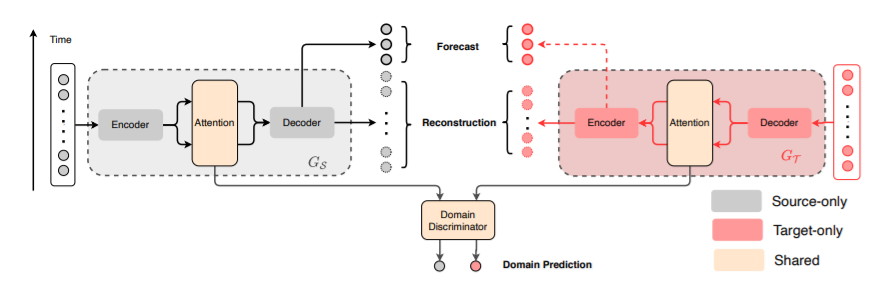
• [1] Private Encoders : privately owned by each domain
  • extract “patterns” & “values”
• [2] Shared Attention
  • compute similarity scores by “domain invariant Q & K” with “patterns”
• [3] Private Decoders : map the attention outputs into “each domain”

(1) Sequence Generator ( \(G_S\), \(G_T\) )

\(G\) processes an input TS \(\mathbf{X}=\left[z_{t}\right]_{t=1}^{T}\), in following order

• 1) private encoders
• 2) shared attention
• 3) private decoder

and outputs..

• output 1) reconstructed sequence \(\hat{\mathbf{X}}\)
• output 2) predicted future \(\hat{\mathbf{Y}}\)

a) Private Encoders

• (input) raw input \(\mathbf{X}\)
• (output)
  • 1) pattern embedding : \(\mathbf{P}=\left[\mathbf{p}_{t}\right]_{t=1}^{T}\)
    • with \(M\) convolutions with various kernel sizes
    • extract “multi-scale local patterns”
  • 2) value embedding : \(\mathbf{V}=\left[\mathbf{v}_{t}\right]_{t=1}^{T}\)
    • with point-wise MLP**
• \(\mathbf{P}\) & \(\mathbf{V}\) are fed into “shared attention module”

b) Shared Attention Module

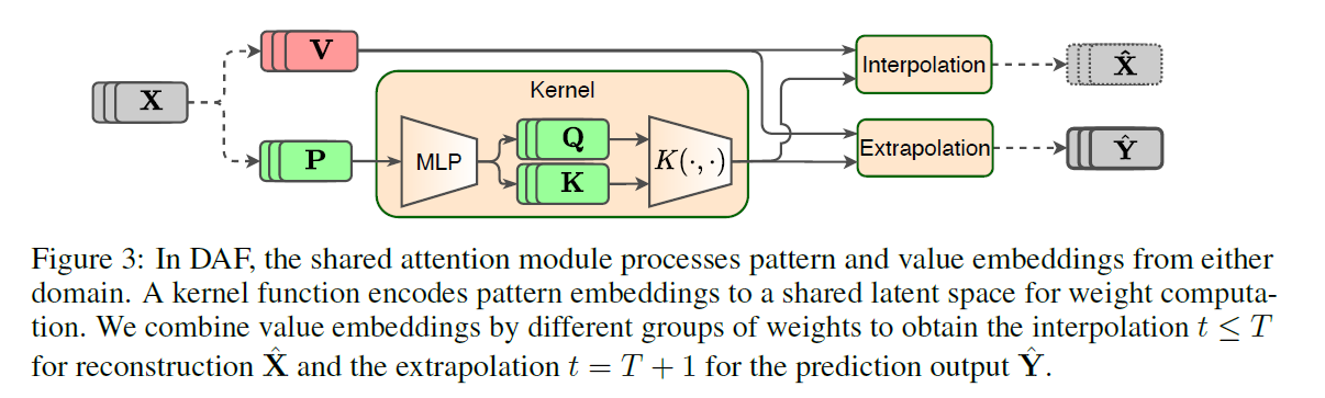
• goal : build QUERY & KEY
  • \(\mathbf{Q}=\left[\mathbf{q}_{t}\right]_{t=1}^{T}\).
  • \(\mathbf{K}=\left[\mathbf{k}_{t}\right]_{t=1}^{T}\).
• how?
  • \(\left(\mathbf{q}_{t}, \mathbf{k}_{t}\right)=\operatorname{MLP}\left(\mathbf{p}_{t} ; \boldsymbol{\theta}_{s}\right)\).
• attention weight :
  • \(\alpha\left(\mathbf{q}_{t}, \mathbf{k}_{t^{\prime}}\right)=\frac{\mathcal{K}\left(\mathbf{q}_{t}, \mathbf{k}_{t^{\prime}}\right)}{\sum_{t^{\prime} \in \mathcal{N}(t)} \mathcal{K}\left(\mathbf{q}_{t}, \mathbf{k}_{t^{\prime}}\right)}\).
  • ex) \(\mathcal{K}(\mathbf{q}, \mathbf{k})=\exp \left(\mathbf{q}^{T} \mathbf{k} / \sqrt{d}\right)\)
• output :
  • \(\mathbf{o}_{t}=\operatorname{MLP}\left(\sum_{t^{\prime} \in \mathcal{N}(t)} \alpha\left(\mathbf{q}_{t}, \mathbf{k}_{t^{\prime}}\right) \mathbf{v}_{\mu\left(t^{\prime}\right)} ; \boldsymbol{\theta}_{o}\right)\).

c) Private Decoders

• (input) \(\mathbf{o}_{t}\)
• (output) \(\hat{z}_{t}\) for each domain
• how?
  • \(\hat{z}_{t}=\operatorname{MLP}\left(\mathbf{o}_{t} ; \boldsymbol{\theta}_{d}\right)\).
• as a result, generate…
  • 1) reconstructions : \(\hat{\mathbf{X}}=\left[\hat{z}_{t}\right]_{t=1}^{T}\)
  • 2) one-step prediction : \(\hat{z}_{T+1}\)

(2) Domain Discriminator

Induce the Q & K of the shared attention module to be domain-invariant

\(\rightarrow\) introduce a domain discriminator \(D: \mathbb{R}^{d} \rightarrow[0,1]\) ( as a position-wise MLP )

• \(D\left(\mathbf{q}_{t}\right)=\operatorname{MLP}\left(\mathbf{q}_{t} ; \boldsymbol{\theta}_{D}\right), D\left(\mathbf{k}_{t}\right)=\operatorname{MLP}\left(\mathbf{k}_{t} ; \boldsymbol{\theta}_{D}\right)\).

Binary classifications

• on whether \(\mathbf{q}_{t}\) and \(\mathbf{k}_{t}\) originate from the source or target
• by minimizing CE loss of \(\mathcal{L}_{\text{dom}}\)

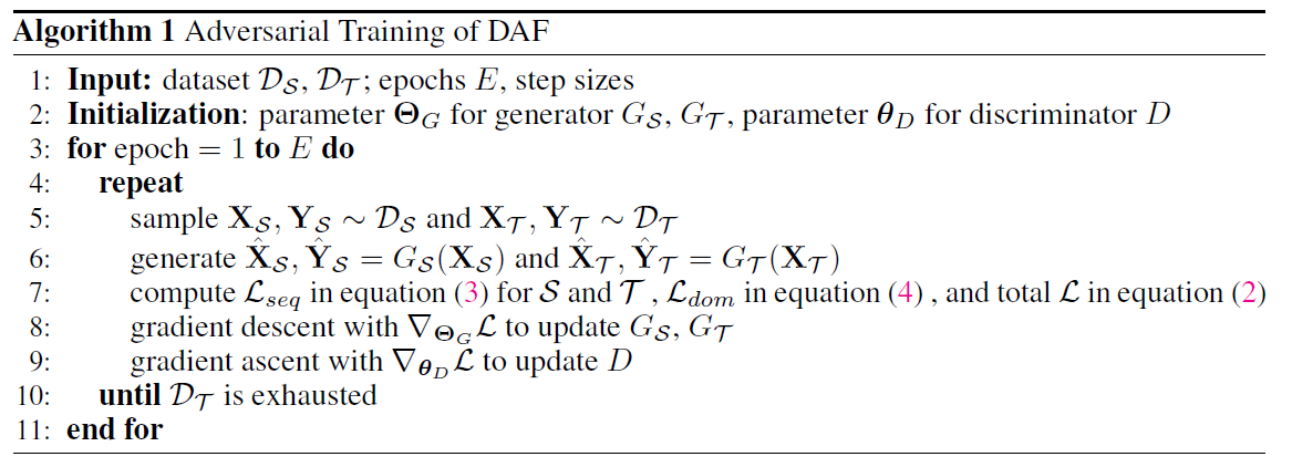
(3) Adversarial Training

Generator \(G_S\), \(G_T\)

• based on private encoder/decoder & shared attention module

Discriminator \(D\)

• induce the invariance of latent features \(\mathbf{K}\) & \(\mathbf{Q}\)