(paper) Multivariate Time Series Anomaly Detection via Graph Attention Network

Multivariate Time Series Anomaly Detection via Graph Attention Network (2020, 44)

Contents

1. Abstract
2. Introduction
3. Related Works
4. Methodology
   1. Overview
   2. Data preprocessing
   3. Graph Attention
   4. Joint Optimization
   5. Model Inference

0. Abstract

Anomaly detection on MTS

• recent approaches : do not capture relationships bewteen TSs

Propose a MULTI-variate TS Anomaly detection

• (1) considers each univariate TS as individual feature
• (2) includes 2 GAT layers in parallel
  • a) for temporal dimensions
  • b) for feature dimensions
• (3) jointly optimizes a
  • a) forecasting-based model
  • b) reconstruction-based model

1. Introduction

essential to consider CORRELATIONS between different TS

Propose MTAD-GAT ( = Multivariate Time-series Anomaly Detection via GAT )

• (1) considers each univariate ts as individual feature

• (2) tries to model the correlations between different features explicitly

2 GAT layers

• (1) feature-oriented
  • capture causal relationshipbs between multiple features
• (2) time-oriented
  • captures dependencies along the temporal dimension

2. Related Works

2 categories of Anomaly Detetion

• (1) individual TS by appyinig univariate models
• (2) multiple TS as a unified entity

2 paradigims of Anomaly Detetion

• (1) forecasting-based
• (2) reconstruction based

Both forecasting & reconstruction based models have supereiority in some situations

\(\rightarrow\) actually, they are complementary!

3. Methodology

Notation

• \(x \in R^{n \times k}\) : input MTS

  • \(n\) : maximum length of timestamps
  • \(k\) : number of features

  ( for a long ts, generate fixed length inputs by a sliding window of length \(n\) )

• \(y \in R^{n}\) : output vctor

  • \(y_{i} \in\{0,1\}\) , whether anomaly or not

Address this problem, by modeling the inter-feature correlations & temporal dependencies,

• with 2 GAT in parallel,

• followed by GRU network

Leverage the power of both (1) forecasting & (2) reconstruction based models

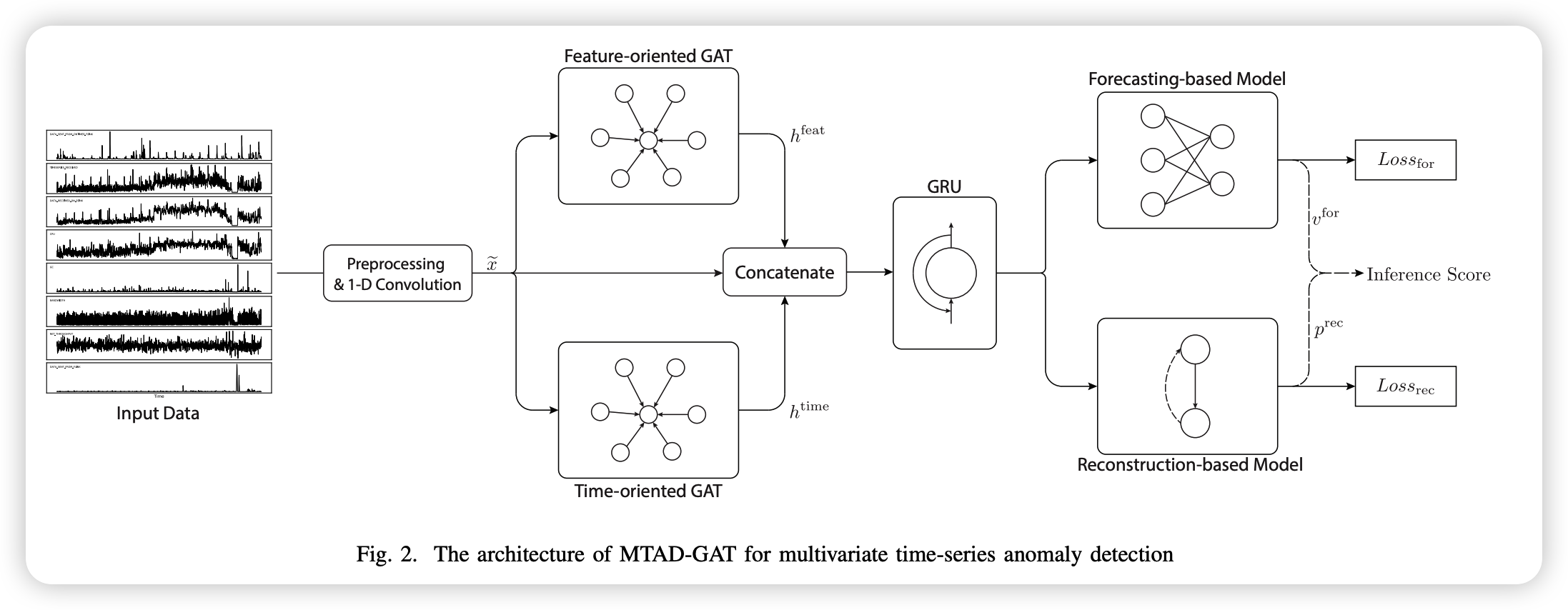
(1) Overview

MTAD-GAT

• step 1) apply 1-d convolution

  • kernel size = 7
  • extract high-level features

• step 2) 2 parallel GAT layers

  • captures relationshipbs between multiple features & timestamps

• step 3) concatenate output & feed to GRU

  • output 1) 1-d conv

  • output 2) two GAT layers

  • feed the concatenated output to the GRU
    • capture sequential patterns

• step 4) feed into forecasting & reconstruction based models

  • Forecasting based model : FC
  • Reconstruction based model : VAE

(2) Data preprocessing

to improve robustness of the model!

1. Data Normalization
2. Data Cleaning

Data Normalization :

• Min-Max noramlization
• Data : both on Training & Testing set

Data Cleaning

• sensitive to irregular & abnormal instances in training set

• use SR (Spectral Residual) to detect anomaly timestamps in each individual TS

  ( threshold of 3 )

• Data : only on Training set

(3) Graph Attention

• \(v_i\) : feature vector of each node
• output representation : \(h_{i}=\sigma\left(\sum_{j=1}^{L} \alpha_{i j} v_{j}\right)\).

Attention score ( \(\alpha_{ij}\) )

• \(e_{i j} =\operatorname{LeakyReLU}\left(w^{\top} \cdot\left(v_{i} \oplus v_{j}\right)\right)\).
• \(\alpha_{i j} =\frac{\exp \left(e_{i j}\right)}{\sum_{l=1}^{L} \exp \left(e_{i l}\right)}\).

(1) Feature Oriented GAT

• detect multivariate correlations
• structure
  • node = ceratin feature ( \(x_{i}=\left\{x_{i, t} \mid t \in[0, n)\right\}\) )
  • edge = relationship between two features
• output shape : \(k\times n\)

(2) Time Oriented GAT

• capture temporal dependencies in time-series
• consider all timestamps wihtin a sliding window as a complete graph
• structure
  • node = feature vector at timestamp \(t\)
  • adjacent nodes = all other timestamps in the current sliding window
• output shape : \(n\times k\)

Concatenate outputs

• a) feature-oriented GAT layer
• b) time-oriented GAT layer
• c) preprocessed \(\tilde{x}\)

\(\rightarrow\) matrix of shape \(n \times 3k\)

(4) Joint Optimization

Model

• (1) forecasting based model : predict the value at next timestamp
• (2) reconstruction based model : capture the data distn of entire time-series

Loss = \(Loss_{forecast} + Loss_{reconstruction}\)

(5) Model Inference

Two inference results for each timestamp

• result 1) prediction value \(\{ \hat{x_i} \mid i=1,\cdots k \}\)
• result 2) reconstruction probability \(\{ \hat{p_i} \mid i=1,\cdots k \}\)

Final inference score ( \(s_i\) )

• balances their benefits, to maximize the overal effectiveness of AD

• calculate \(s_i\) for each feature,

  take summation of all features \(\rightarrow\) final score

• anomaly if inference score is larger than a threshold

\(\text { score }=\sum_{i=1}^{k} s_{i}=\sum_{i=1}^{k} \frac{\left(\hat{x}_{i}-x_{i}\right)^{2}+\gamma \times\left(1-p_{i}\right)}{1+\gamma}\).