(paper) Time Series Forecasting with Deep Learning ; A Survey

Time Series Forecasting with Deep Learning : A Survey (2020)

Contents

1. Abstract
2. DL for ts forecasting
   1. Basic Building Blocks
   2. CNN
   3. RNN
   4. Attention
3. Outputs and Loss Functions
   1. Point Estimates
   2. Probabilistic Outputs
4. Multi-horizon Forecasting models
   1. Iterative Methods
   2. Direct Methods
5. Incorporate Domain Knowledge with Hybrid Models
   1. Non-probabilistic Hybrid Models
   2. Probabilistic Hybrid Models

0. Abstract

survey encoder & decoder design used in both..

• 1) one-step ahead
• 2) multi-horizion time series forecasting

describe how temporal information is incorporated into predictions

1. DL for ts forecasting

predict future value of \(y_{i, t}\)

one-step-ahead forecasting models

• \(\hat{y}_{i, t+1}=f\left(y_{i, t-k: t}, \boldsymbol{x}_{i, t-k: t}, \boldsymbol{s}_{i}\right)\).
  • model forecast : \(\hat{y}_{i, t+1}\)
  • observations of ( over a look-back window \(k\) )
    • target : \(y_{i, t-k: t}=\left\{y_{i, t-k}, \ldots, y_{i, t}\right\}\)
    • exogenous inputs : \(\boldsymbol{x}_{i, t-k: t}=\left\{\boldsymbol{x}_{i, t-k}, \ldots, \boldsymbol{x}_{i, t}\right\}\)

(1) Basic Building Blocks

basic building blocks = Encoder & Decoder

• construct intermediate feature representations

  ( = encoding relevant historical information into a latent variable \(\boldsymbol{z}_{t}\) )

  \(\boldsymbol{z}_{t}=g_{\mathrm{enc}}\left(y_{t-k: t}, \boldsymbol{x}_{t-k: t}, \boldsymbol{s}\right)\).

• Final forecast produced using \(\boldsymbol{z}_{t}\) alone:

  \(f\left(y_{t-k: t}, \boldsymbol{x}_{t-k: t}, \boldsymbol{s}\right)=g_{\mathrm{dec}}\left(\boldsymbol{z}_{t}\right)\).

(2) CNN

• extract local relationships ( invariant across spatial dimensions )

• use multiple layers of causal convolutions

  ( = ensure only PAST information is used for forecasting )

• \(\boldsymbol{h}_{t}^{l+1}=A((\boldsymbol{W} * \boldsymbol{h})(l, t))\).
• \((\boldsymbol{W} * \boldsymbol{h})(l, t)=\sum_{\tau=0}^{k} \boldsymbol{W}(l, \tau) \boldsymbol{h}_{t-\tau}^{l}\).

Dilated Convolutions

• standard CNN = computationally challenging, where long-term dependencies are significat

• to solve this…

  use dilated convolutional layers

• \((\boldsymbol{W} * \boldsymbol{h})\left(l, t, d_{l}\right)=\sum_{\tau=0}^{\left\lfloor k / d_{l}\right\rfloor} \boldsymbol{W}(l, \tau) \boldsymbol{h}_{t-d_{l} \tau}^{l}\).

  • \(d_{l}\) : layer-specific dilation rate

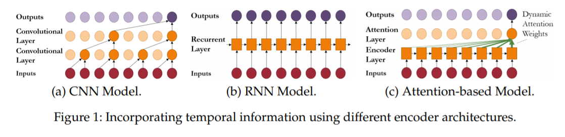
(3) RNN

생략

(4) Attention

Transformer architectures achieve SOTA

• allow the network to directly focus on significant time steps in the past!

  ( even if they are very far back )

• \(\boldsymbol{h}_{t}=\sum_{\tau=0}^{k} \alpha\left(\boldsymbol{\kappa}_{t}, \boldsymbol{q}_{\tau}\right) \boldsymbol{v}_{t-\tau}\).

Benefits of using attention in time series

• use attention to aggregate features extracted by RNN encoders
• \(\boldsymbol{\alpha}(t) =\operatorname{softmax}\left(\boldsymbol{\eta}_{t}\right)\).
  • \(\boldsymbol{\eta}_{t} =\mathbf{W}_{\eta_{1}} \tanh \left(\mathbf{W}_{\eta_{2}} \boldsymbol{\kappa}_{t-1}+\mathbf{W}_{\eta_{3}} \boldsymbol{q}_{\tau}+\boldsymbol{b}_{\eta}\right)\).

2. Outputs and Loss Functions

(1) Point Estimates

\[\begin{aligned} \mathcal{L}_{\text {classification }} &=-\frac{1}{T} \sum_{t=1}^{T} y_{t} \log \left(\hat{y}_{t}\right)+\left(1-y_{t}\right) \log \left(1-\hat{y}_{t}\right) \\ \mathcal{L}_{\text {regression }} &=\frac{1}{T} \sum_{t=1}^{T}\left(y_{t}-\hat{y}_{t}\right)^{2} \end{aligned}\]

(2) Probabilistic Outputs

understand uncertainty of a model’s forecast

common way to model uncertainties :

\(\rightarrow\) use DNN to generate parameters of known distributions

\[y_{t+\tau} \sim N\left(\mu(t, \tau), \zeta(t, \tau)^{2}\right)\]

• \(\mu(t, \tau)=\boldsymbol{W}_{\mu} \boldsymbol{h}_{t}^{L}+\boldsymbol{b}_{\mu}\).

• \(\zeta(t, \tau) =\operatorname{softplus}\left(\boldsymbol{W}_{\Sigma} \boldsymbol{h}_{t}^{L}+\boldsymbol{b}_{\Sigma}\right)\).

  ( to take only positive values )

3. Multi-horizon Forecasting models

beneficial to have estimates at multiple points

• single point : 수요일 예측하기
• multiple points : 수요일/목요일/금요일 예측하기

just slight modification of one-step ahead prediction

• \(\hat{y}_{t+\tau}=f\left(y_{t-k: t}, \boldsymbol{x}_{t-k: t}, \boldsymbol{u}_{t-k: t+\tau}, \boldsymbol{s}, \tau\right)\).

  where \(\tau \in\left\{1, \ldots, \tau_{\max }\right\}\)

  ( 여기서 \(\tau\)가 1이면 one-step ahead prediction )

크게 2 종류의 methods

• 1) Iterative Methods
• 2) Direct Methods

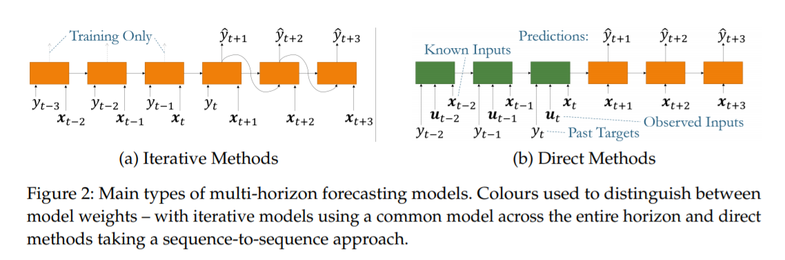
(1) Iterative Methods

• autoregressive DL architectures

  ( produce multi-horizon forecasts by RECURSIVELY feeding samples of the target into future steps )

• by repeating the generation….

  • \[y_{t+\tau} \sim N\left(\mu(t, \tau), \zeta(t, \tau)^{2}\right).\]
  • prediction means : \(\hat{y}_{t+\tau}=\sum_{j=1}^{J} \tilde{y}_{t+\tau}^{(j)} / J\).

(2) Direct Methods

• produce forecasts directly using all available inputs

• seq2seq architectures

4. Incorporate Domain Knowledge with Hybrid Models

Hybrid Methods = (1) + (2)

• (1) well studied quantitative t.s. model
• (2) DL

Characteristics

• allow domain experts to inform NN using prior information

• especially useful for small datasets

• allow for separation of (1) stationary & (2) non-stationary components
• avoid the need for custom input pre-processing

Example : ESRNN (Exponential Smoothing RNN)

• exponential smoothing to capture non-stationary trends
• learn additional effects with RNN

How is DL used?

• 1) encode time-varying parameters for non-probabilistic parametric models
• 2) produce parameters of distributions used by probabilistic models

(1) Non-probabilistic Hybrid Models

ESRNN 소개

• 1) utilizes the update equations of Holt-Winters exponential smoothing model

• 2) combine multiplicative level & seasonality components with DL outputs

• 수식
  • \(\hat{y}_{i, t+\tau} =\exp \left(\boldsymbol{W}_{E S} \boldsymbol{h}_{i, t+\tau}^{L}+\boldsymbol{b}_{E S}\right) \times l_{i, t} \times \gamma_{i, t+\tau}\).
    • \(l_{i, t} =\beta_{1}^{(i)} y_{i, t} / \gamma_{i, t}+\left(1-\beta_{1}^{(i)}\right) l_{i, t-1}\).
    • \(\gamma_{i, t} =\beta_{2}^{(i)} y_{i, t} / l_{i, t}+\left(1-\beta_{2}^{(i)}\right) \gamma_{i, t-\kappa}\).

(2) Probabilistic Hybrid Models

produce parameters for predictive distn at each step

ex) Deep State Space Models

• encode time-varying parameters for linear stat space models

  ( perform inference via Kalman filtering equations )

• \(y_{t} =\boldsymbol{a}\left(\boldsymbol{h}_{i, t+\tau}^{L}\right)^{T} \boldsymbol{l}_{t}+\phi\left(\boldsymbol{h}_{i, t+\tau}^{L}\right) \epsilon_{t}\).

  • \(\boldsymbol{l}_{t} =\boldsymbol{F}\left(\boldsymbol{h}_{i, t+\tau}^{L}\right) \boldsymbol{l}_{t-1}+\boldsymbol{q}\left(\boldsymbol{h}_{i, t+\tau}^{L}\right)+\boldsymbol{\Sigma}\left(\boldsymbol{h}_{i, t+\tau}^{L}\right) \odot \boldsymbol{\Sigma}_{t}\).